Introduction
Soil is the basis of agricultural production. A healthy soil is an essential component of a healthy environment; it is the foundation upon which a sustainable agriculture production system is built. Healthy soils are productive, resilient to stressors, and more resistant to degradation.
Soil health refers to the soil’s ability “to support crop growth without becoming degraded or otherwise harming the environment” (Agriculture and Agri-Food Canada). It is typically evaluated by examining chemical, physical, and biological properties that serve as indicators of how well the soil functions to provide services such as supporting crop production. Other approaches to assessing soil health involve evaluating the risks of specific soil degradation threats such as erosion or compaction.
The Soil Health Assessment and Plan (SHAP) is a tool to guide farmers and their advisors in identifying soil health challenges and management practices to address them. SHAP can be used to create a soil health baseline for future monitoring, or to compare different fields or sections of fields to one another. It provides a variety of soil health assessment modules, including risk assessment tools, in-field observations, and laboratory tests to identify soil health challenges, as well as indexes for evaluating soil management practices. These modules give the user the flexibility to determine the scope and level of detail of the assessment.
The ultimate result of SHAP is a soil health management plan tailored to the soil and production system of each farm. The more modules completed, the more comprehensive and specific the management plan can be.
Our understanding of soil health is still evolving. As the science advances, this tool may change to accommodate new knowledge and soil assessment methods.
If you have any questions, comments, or suggestions for improvements, please contact the author.
How to use this guide
This guidebook will lead you through conducting the Soil Health Assessment and Plan (SHAP). It is divided into three sections that relate to the technical elements and steps involved in SHAP.
- Part 1 – Using the Tool: explains where to start with SHAP – defining the goal for the assessment and using that goal to determine the assessment approach that will meet your needs. It also provides instructions for using the Survey123 app to collect the necessary information and for performing the assessment modules.
- Part 2 – What to do in the Field: provides instructions for collecting in-field observations and soil samples for analysis.
- Part 3 – Results Interpretation and Planning Guide: provides guidance on interpreting the results of the assessments in SHAP and recommending beneficial management practices, as well as guidelines for preparing a report.
Part 1 – Using the Tool
Before you start
The SHAP process
Soil health describes the interaction between inherent soil properties and management. It is dynamic and can change over time as it responds to management or as management changes. SHAP collects information about the soil and the way it is managed, measures soil health indicators, and provides a framework for integrating and interpreting the information to improve soil management and soil health. The sections of this guidebook mirror the steps of the SHAP process:
- Collecting the information
- Collecting samples and performing the assessments in the field
- Interpreting the data and formulating a management plan
Organic (muck) soils
Organic soils (> 30% organic matter by weight) are very different from mineral soils in their properties and behaviour. SHAP is not intended for use in organic soils.
The SHAP Test
The SHAP Test is the foundation of SHAP and includes the lab tests for the following analytical indicators:
- Soil organic matter
- Active carbon
- Soil respiration
- Potentially mineralizable nitrogen
- Aggregate stability
Combined, these provide information on the biological and physical health of soil and complement the information provided by a standard soil fertility (chemical) test. SHAP results are compared to a database of Ontario soils and scored against soils of the same textural class. More information on the indicators in SHAP can be found in Part 3 of this guidebook.
For a list of labs currently offering the SHAP testing package, see: Participating Soil Testing Labs
Although soil fertility is an integral part of soil health and crop production, SHAP does not include soil fertility analyses. Recent soil fertility values for pH, phosphorus and potassium are requested as a part of SHAP to ensure that important, productivity-limiting concerns are not over-looked, but SHAP does not replace or repeat existing tools for evaluating soil fertility.
Determine the assessment objective(s) and location(s)
Define the goal of the assessment
Different users will have different goals when undertaking a soil health assessment. Common goals include:
- setting a benchmark to compare to future assessments for identifying trends
- understanding the most important limitations and risks to the soil’s productivity
- comparing good and poor areas of a field
Defining a goal for the assessment will make it easier to decide which modules to include, and whether to take one sample representing the average of one field or multiple samples in different zones or fields.
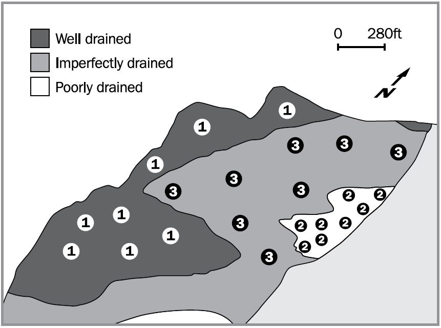
Select a field
Not all fields perform equally, and variability also exists within the boundaries of a field. This variability must be accounted for in selecting fields and sites to sample. Consider the goal that was stated and decide which field and what area(s) within it should be sampled to support the goal. The following table provides some examples as guidance.
| Field | Description and rationale |
| Poor | Consistently produce below-average yields and may be limited by soil factors such as compaction, drainage problems, or erosion. Identifying the issue can help in developing a plan to make the field more productive. |
| Average | Representative of most acres in an operation. Select to make the results of the assessment broadly applicable to the rest of the farm operation. |
| New | Fields that have been recently purchased or improved. They are good candidates for benchmarking to understand how adoption of soil health management practices will impact soil over time. |
| Good | Consistently perform above the farm average. Assessing such fields can provide a target to aim for when evaluating “Poor”, “Average” or “New” fields with similar soils. |
Select the sampling location(s)
Once a field has been chosen, it is important to select a suitable location within it. Since SHAP currently functions primarily for benchmarking and comparison, it is suggested that sampling and observations are performed in a relatively small area. Results should not be extrapolated to other areas of the field.
If good data exists for the field (e.g. yield index maps, soil property maps) or if reliable management zones have been established, this information can guide the selection of a sampling location(s) within the field.
If this is not the case, consider using a topography or performance-based approach. The table below may be used for guidance.
| Selection Criteria | Site Characteristics | Description |
|---|---|---|
| Topography | Lower slope position | Water flows to and accumulates in these areas. |
| Typically poorly drained soils, often finer (heavier) textured. | ||
| Typically highly productive if tile drained, but excessive moisture can be an issue in some years. | ||
| Mid slope position | Generally intermediate crop productivity in sloping fields. | |
| Typically well to imperfectly drained soils. | ||
| May experience water and/or tillage erosion. | ||
| Upper slope position | Generally drier areas of the field. | |
| Typically well to rapidly drained soils. | ||
| Knolls and shoulder slopes likely significantly eroded and at high risk of further tillage erosion. | ||
| Performance | Below average-yielding | May be limited by soil factors or by degradation such as compaction, erosion, or low organic matter. |
| Comparing to higher-yielding areas may help identify the issues to develop a remediation plan and improve productivity. | ||
| Average-yielding | Broadly representative of the field. | |
| May be used to make the results of the assessment more generally applicable to the field. | ||
| High-yielding | Represents the best potential of similar soil in the field. | |
| May be used to compare against low- or average-yielding areas. | ||
| Inconsistent | Yields are high in some years and low in others. | |
| Often attributable to soil moisture fluctuations. |
Select the right modules
Just the Test
For a simple, laboratory-based analysis of soil health that doesn’t involve apps and requires minimal additional information, the SHAP Test can be performed on its own. The SHAP Test is simply the suite of lab tests included in SHAP. Lab results can be scored and interpreted using the same approach, as outlined in Part 3.
Users who are only interested in the SHAP Test can use the app and select “no additional modules”. Those looking to skip the app altogether can simply include the SHAP Submission Form when sending soil samples in to participating soil testing labs.
However, SHAP works best as a comprehensive tool that combines information on soil characteristics, management, and indicators of interest in a format that guides users through interpretation of results and planning to address challenges. For a fuller understanding of soil health, it is recommended to use the SHAP Tool and complete as many SHAP modules as possible.
For the list of analyses in the SHAP Test, see: SHAP Test
For a list of labs currently offering the SHAP Test, see: Participating Soil Testing Labs
For a copy of the fillable submission form, follow this link: SHAP Submission Form
SHAP Modules
SHAP also includes several optional modules in the SHAP Tool in addition to the basic assessment. These provide additional information and different perspectives on soil health and soil management. These modules currently include:
Management Evaluations
- Tillage disturbance index – rates the tillage system by the intensity of soil disturbance
- Living roots index – measures the proportion of the year with living roots in the soil
Risk Assessments
- Water erosion risk assessment – calculates risk of water erosion across a field based on landscape, tillage, and cropping factors
- Compaction risk assessment – estimates risk of subsurface compaction from equipment and soil characteristics
In-field Assessments
- Soil structure assessment – scores the quality of the surface and topsoil structure
SHAP Test or SHAP Tool?
The SHAP Test is included in the SHAP Tool. The SHAP Tool makes it easy to link results to a specific location in the field, and to collect information about soil and management system characteristics that provide important context for interpreting those results and developing the management plan in the SHAP report. The tool automatically fills a SHAP report template with all the information entered in the tool and the outputs generated from the optional modules.
| SHAP Test | SHAP Tool | |
|---|---|---|
| Lab tests of soil health indicators | x | x |
| Optional add-on modules for evaluating soil health, management, and risks | x | |
| Integration with Ontario soil map data | x | |
| Mobile-friendly data collection forms | x | |
| Auto-generated report template | x |
The SHAP Tool
Using the App (Survey123)
Survey123 is an ArcGIS online application that is used for SHAP because it can connect to Ontario soil map data in the background. It can be accessed on a computer through a browser (e.g., Google Chrome) or by downloading the desktop app. It can also be downloaded as an app on smartphones and tablets for field data collection.
Computer or Mobile?
Survey123 can be used on either a computer or a mobile device, but it’s not possible to switch between them for the same survey. A computer is required for the risk assessment modules in the Soil Management survey because these use external tools and require switching between those tools and Survey123.
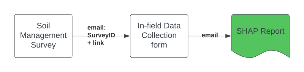
The SHAP Tool is divided into two parts:
- Soil Management survey
- In-Field Data Collection form
The two parts are linked in Survey123 by a survey ID generated from the submitter’s initials and the name of the field being assessed. This makes it possible to perform the Soil Management survey on the computer and then transition to a mobile device to complete the In-field Data Collection form.
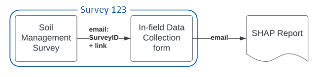
The Soil Management survey collects background information on the field, soil, and management system. Optional management and risk assessment modules are included here if selected. It is strongly recommended to complete this survey on a computer. If the Water Erosion Risk module is selected this survey can only be done on a computer as the tool that runs the module is not available on mobile browsers. It’s important that the Soil Management survey be completed and submitted first so that the information can be properly connected to the field data.
The In-field Data Collection form is used for collecting information about the sampling site, including the optional soil structure evaluation modules. You will need a GPS for this survey, either integrated in the device (e.g., most smartphones) or externally connected (e.g., a GPS receiver connected to a computer).
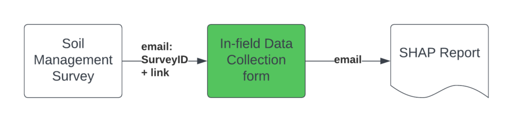
Once you submit the Soil Management survey you will receive an email with a link to the In-Field Data Collection form. This email will also generate a unique Survey ID that must be entered exactly in the In-Field Data Collection form so that it can be connected to the right Soil Management survey.
Once both the Soil Management survey and the In-field Data Collection form have been completed and submitted, the submitter will receive an emailed SHAP report template containing the information gathered throughout the tool.
When you’re ready to start, click on the link below to open the Soil Management survey in Survey123.
Soil Management Survey
Module selection
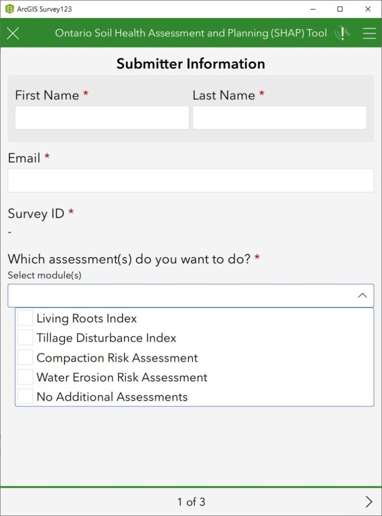
The optional add-on modules are hidden until selected, so it’s important to select these modules from the start as they will change the flow of the tool and the forms for several input categories.
Management Evaluations
- Tillage disturbance index – rates the tillage system by the intensity of soil disturbance
- Living roots index – measures the proportion of the year with living roots in the soil
Risk Assessments
- Water erosion risk assessment – calculates risk of water erosion across a field based on landscape, tillage, and cropping factors
- Compaction risk assessment – estimates risk of subsurface compaction from equipment and soil characteristics
In-field Assessments
- Soil structure assessment – scores the quality of the surface and topsoil structure
Describing Soil Health Challenges and Goals
Experience and observations of soil performance within and between fields can provide insight into potential soil health problems or trends that may not be apparent at the time of a field visit. Consider any soil-related limitations to production (e.g., drainage issues, variability, disease, fertility, etc.) or trends that have been observed over time (e.g., soil organic matter levels, crop yields and yield stability). This helps set an observable benchmark to compare with future follow-up soil health assessments.
Setting a soil health goal can help to guide management recommendations or to prioritize among multiple recommended options. Reviewing the goal during follow-up assessments also provides another way to measure progress. The goal could directly relate to the soil health challenges, or more generally relate to how a farmer wants their soil to “work” in their production system.
Field and Soil Information
Field Information
Enter a field name that makes sense to you. It will be included in the Survey ID generated to connect the Soil Management survey with the In-field Data Collection survey.
Select from the lists the reasons why this field was selected, and what soil health challenges you have experienced on it.
Write out your soil health goal for this field. This will be an important marker to evaluate the success of your management plan when you revisit the SHAP report in the future.
Soil Information
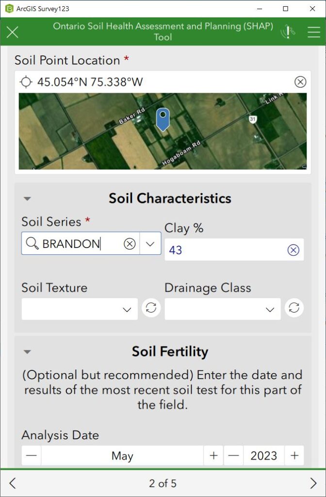
Use the map service to view the names of soil types in the field from soil maps. If you are at the field and location services are enabled on your device, click the target icon ![]() under Soil Point Location to automatically zoom to your location. Otherwise, click the map icon
under Soil Point Location to automatically zoom to your location. Otherwise, click the map icon  to pan and zoom to the field. Drop a point anywhere in one of the soil polygons in the field by panning the map and clicking the check at the bottom right corner. (See the box “Soil Maps” if you do not see the soil polygons.)
Enter the name of the soil series – the soil series list is filtered based on the letters typed in the box. Click on the refresh icon ![]() to fill any empty soil characteristics. Clay % represents the clay content at 35 cm depth of a representative profile for the recorded soil series and is used in the compaction risk assessment module.
to fill any empty soil characteristics. Clay % represents the clay content at 35 cm depth of a representative profile for the recorded soil series and is used in the compaction risk assessment module.
Soil Maps
The soil map layer should appear once the map is zoomed in to the field. If the soil map layer does not appear when zoomed in, click on the base map icon (top of the right-hand side bar) and select the ‘Ontario Soil Health Assessment and Planning Tool’ basemap.
Enter the soil fertility information associated with the point. If the field has not been grid or zone sampled, enter the soil test results for the field. Otherwise, select the fertility ranges that best correspond to the point location.
Repeat this process with every significant (>10% of field area) soil polygon in the field by clicking the  icon at the bottom right of the page.
Crop and Soil Management System
Collecting information about the cropping system provides baseline information to evaluate potential problems or areas for improvement in the soil management system. This information is the starting point for the recommendations in the Soil Health Management Plan.
NOTE: The following section is modified if the Living Roots Index or Tillage Disturbance Index are selected.
Crop Management System (no additional modules)
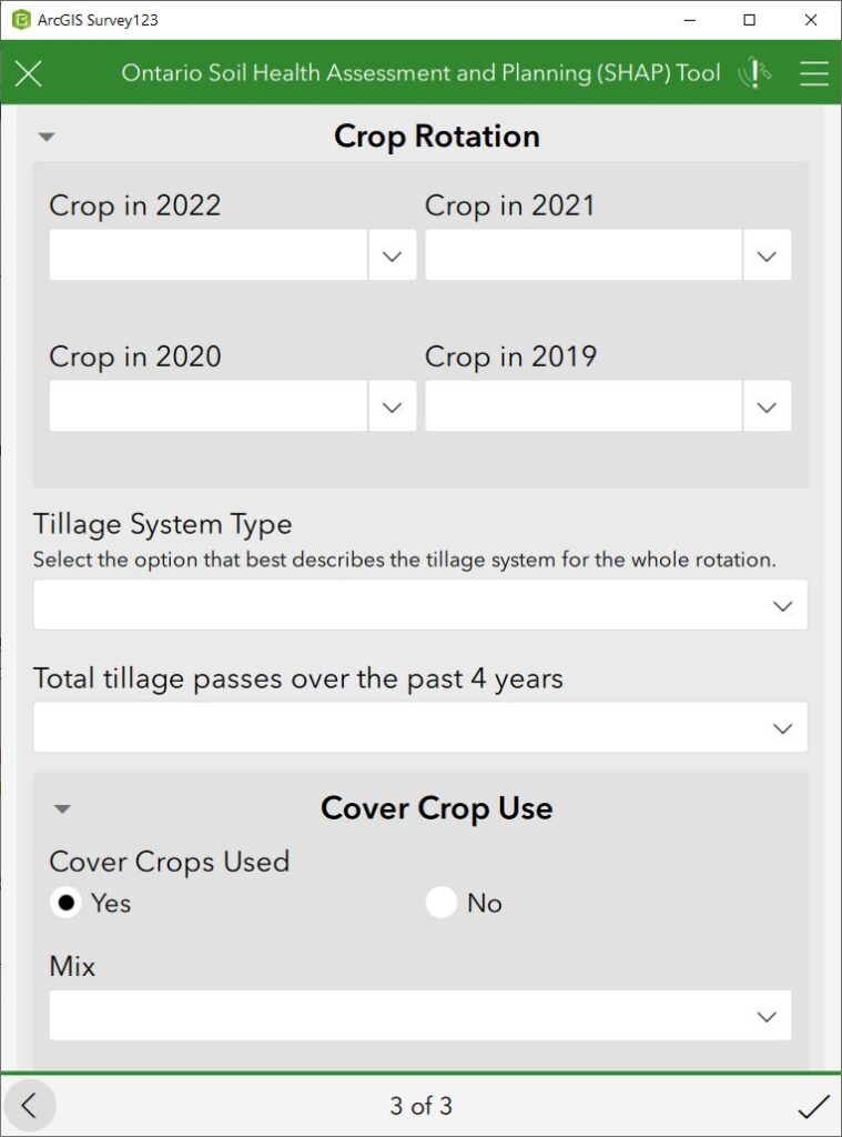
Enter the crops grown in the previous 4 years in this field. Typing the first few letters of the crop will filter the list.
Select the option that best describes your tillage system over the past 4 years, and enter the sum of all the tillage passes over the same period.
If you use cover crops, select the options that best describe the mix and species type(s) used, and select all the termination methods and timings that apply.
If you use organic amendments, select the type and describe how often they are applied.
Finally, add any additional comments that provide important context (e.g., “regular manure additions until 5 years ago”)
Crop Management System (Living Roots Index module)
The Living Roots Index provides a measure of the average number of days per year with living roots in the soil, an important metric for managing soil health. This average requires at least four years of cropping date information to be calculated.
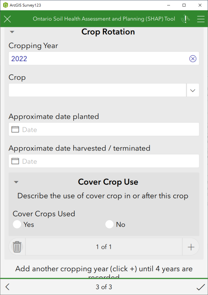
Build the crop rotation history by adding the four most recent completed cropping years. Add a cropping year by clicking the plus icon . The default cropping year is last year. Depending on the date and/or current crop, that cropping year may not be completed. Make sure to start with the most recent completed cropping year.
For a given cropping year, select the crop grown. Typing the first few letters of the crop will filter the list. Record the approximate date the crop was planted and harvested. (Note: the calendar date selector defaults to the current date.) If cover crops were grown that year, describe the cover crop system and approximate dates of seeding and termination.
Click the plus icon ![]() to add another cropping year and repeat the steps above until four cropping years have been described.
to add another cropping year and repeat the steps above until four cropping years have been described.
Unless the Tillage Disturbance Index module was selected, describe the tillage system and organic amendment use as in the basic module.
Crop Management System (Tillage Disturbance Index module)
The Tillage Disturbance Index provides a quantitative measure of the intensity of tillage disturbance to the soil over the crop rotation. It uses the soil tillage intensity rating (STIR) system developed for the Revised Universal Soil Loss Equation (RUSLE2). It is calculated for each cropping year and then averaged over 4 years. The Tillage Disturbance Index requires details about the use of each tillage implement used in the previous 4 years.
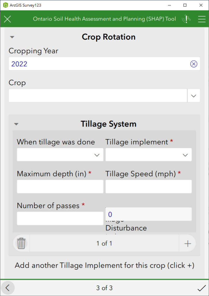
For a given cropping year, select the crop grown. Typing the first few letters of the crop will filter the list. For each tillage implement used in or before that crop, describe the timing, type of implement, maximum depth, average speed, and number of passes.
If there was no tillage done, select “not applicable” as the timing. Select as tillage implement “no disturbance (perennial)” for perennial crops, or “no-till” direct-seeded crops. The other variables should auto-populate to 0. Otherwise click the refresh icon ![]() or enter 0 manually.
or enter 0 manually.
Some tillage implements (e.g., strip till, subsoiling) will also require a percentage of the soil surface disturbed – think of this as the proportion of the working width of the tool that is actually tilled (see the box Area disturbed for an example). Click the plus icon ![]() to add any other tillage implement used in or before that crop.
to add any other tillage implement used in or before that crop.
Click the plus icon ![]() to add another cropping year and repeat the steps above until four cropping years have been described.
to add another cropping year and repeat the steps above until four cropping years have been described.
Area disturbed
Bob strip tills his corn – what % of the field area is worked? You can calculate this from row spacing and strip width.
Bob plants corn on 30 in rows, and his strip till rig makes strips 8 in wide. The % area disturbed by Bob’s strip till pass is equal to the width of the strip divided by the distance between strip centres, multiplied by 100.
A = (8 in / 30 in) * 100 = 27%
Risk Assessment Modules
Water Erosion Potential
The Water Erosion Potential Map estimates water erosion risk based on soil type, topography, tillage system and crop rotation. It performs calculations from the Revised Universal Soil Loss Equation (RUSLE2) using data from the most recent soil maps for soil and landscape factors and calculates a ‘conservation’ (C) factor using tillage and cropping information provided by the user.
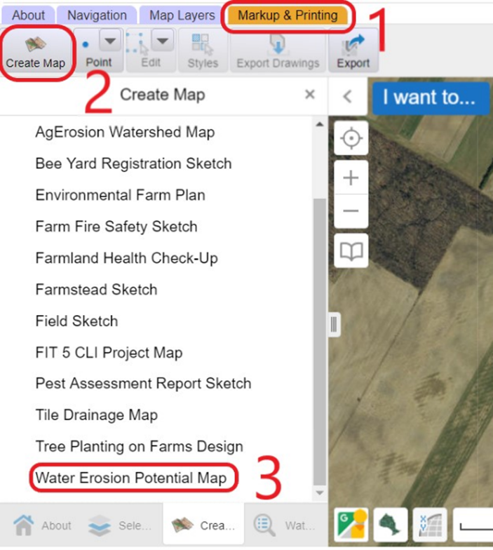
Step 1. Navigate to the tool
- Click on the “AgMaps” link in Survey123, or click here
- Once you have opened AgMaps, click on the ‘Markup and Printing’ tab
- Click the ‘Create Map’ button and scroll down to ‘Water Erosion Potential Map’
Step 2. Select the field
- Navigate to the field on the map. You may want to switch to satellite imagery view (click the
 icon at the bottom of the map) as you get closer
 - Once the field is on the screen, click the polygon button under ‘Field Boundary / Area of Interest’
- To outline the field: click on a corner of the field then click again on the next corner to end a line. Continue until the last corner. To complete the outline, double click the last corner – the line between your last and first points will be created automatically to complete the polygon.
- Enter the farm and field name
- The tool will now automatically calculate the inherent water erosion potential (the amount of erosion that would occur if the field were left bare for a year)
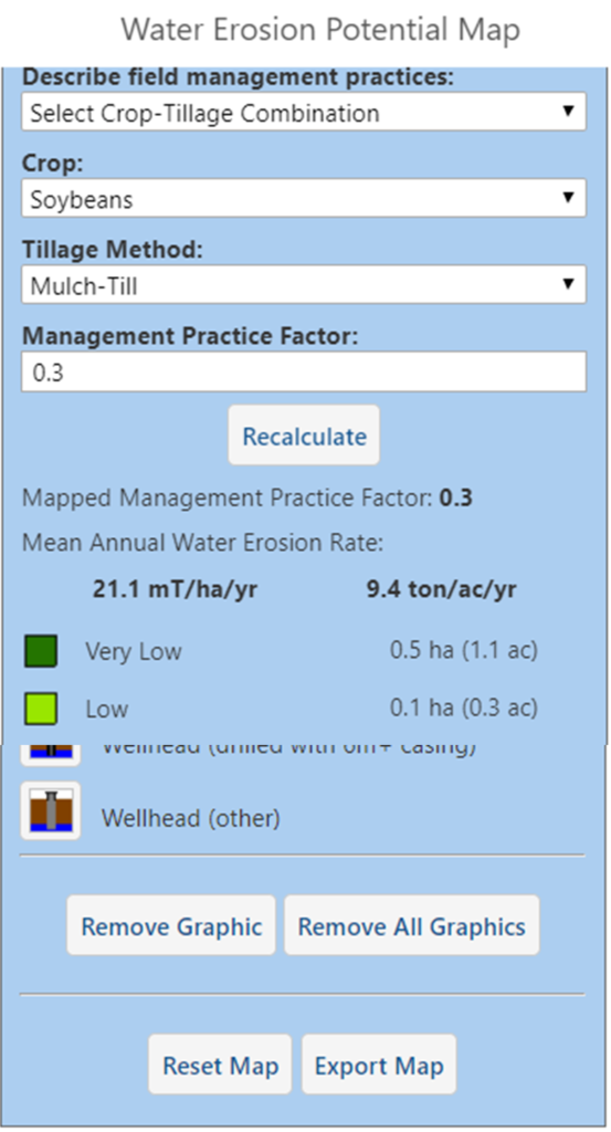
Step 3. Determine C factor
- In the left sidebar, click “Display Mean Annual Water Erosion Estimate Map” under Map Display Options.
- Under “Describe field management practices” select “Select Crop-Tillage Combination”
- Select the crop that leaves the lowest amount of residue after harvest (e.g., corn silage, soybeans) and the tillage method used to prepare for its planting, and click the “Recalculate” button
- Save the file as a PDF or Picture by pressing the “Export Map” button at the bottom of the left sidebar and upload this file in Survey 123 by clicking the paperclip icon.
Step 4. Record results
In Survey123, enter the area of the field experiencing moderate, high, and very high Mean Annual Water Erosion Rate, as well as the total field area (scroll up to find it under the field name in the sidebar of the Water Erosion Potential Map). The survey will automatically calculate the proportion of the field with an elevated risk of erosion.
Compaction risk assessment (Terranimo)
Terranimo is a compaction risk assessment tool developed by soil scientists at the University of Bern in Switzerland that allows you to understand how soil conditions and machinery parameters influence the risk of compaction.
This assessment should be run based on the highest risk scenario for a given field, i.e., the highest clay content in the field and the heaviest equipment used. In Ontario, high risk conditions of moist to very moist soil typically occur during spring/planting and fall/harvest season operations.
The purpose of this section of the survey is to collect the information about an operation’s equipment and use that is needed to use Terranimo for estimating the risk of subsoil compaction damage and creating a compaction avoidance plan.
Equipment Characteristics
Select the type that best describes the heaviest piece of equipment that goes over the field. Enter its total weight in kg when loaded (i.e., the towing load, the sum of the curb weight and load weight), the number of axles, and total number of wheels.
Tire Characteristics
Describe the tires on the heaviest axle of the equipment. The type, make, model, and size are necessary for finding the manufacturer’s recommendations on inflation pressure and load. Enter the tire pressure in psi – the survey will automatically convert this to bar for use in Terranimo and will also calculate the axle load and wheel load.
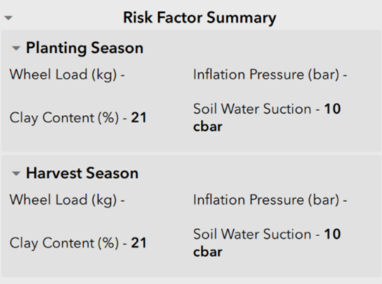
Risk Factor Summary
This section presents a summary of the equipment and soil information that will be entered into Terranimo.
Using Terranimo
Repeat the following steps for both spring/planting and fall/harvest season:
Step 1. Navigate to the tool
Click on the “Terranimo” link in Survey123 or go to https://ch.terranimo.world/light (to switch to English – click “EN” in the top right corner).
Light or Expert?
Currently, SHAP uses the “light” version of Terranimo as Ontario soil profile data is not available in the tool. The “expert” version produces a more informative result but requires more detail about equipment characteristics and soil properties by layer.
Step 2. Estimate compaction risk from soil and equipment characteristics
Enter the wheel load (kg), inflation pressure (bar), maximum clay content within the field (%) and soil water suction from the Risk Factor Summary into Terranimo.
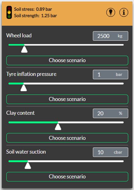
Soil water suction is set to 10 cbar as this represents the wetter end of the “moist” range. Many time-sensitive field operations are done when the soil is not quite “fit” yet, so this is a reasonable setting for to describe the high-risk scenarios that are common in the shoulder seasons in Ontario.
Step 3. Record the ratio of soil strength to soil stress
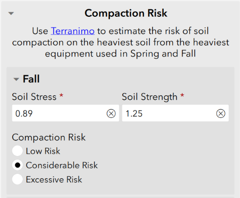
From the coloured bar at the top of the Terranimo sidebar, enter the estimates of soil stress and soil strength (e.g., 0.89 and 1.25 respectively in the example given) into Survey 123. Click the refresh icon ![]() if the risk level is not automatically computed.
if the risk level is not automatically computed.
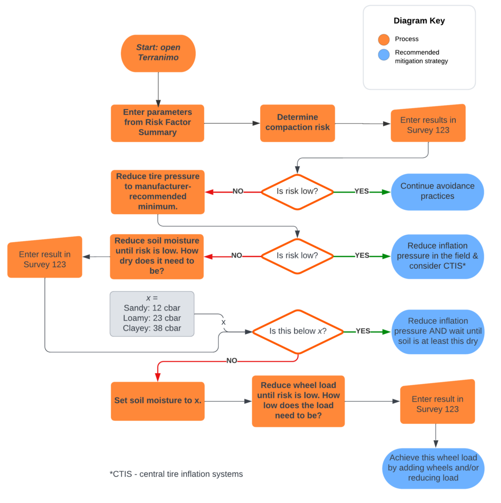
Step 4. Create a compaction avoidance plan
If the risk level is not low, the survey will prompt additional actions to determine how to reduce compaction risk. The instructions and flowchart below outline the options, in order of increasing change from the current practice.
- Reducing tire pressure
- Use the tire characteristics entered above to find the manufacturer-recommended minimum inflation pressure for the wheel load calculated in the risk factor summary.
- Enter this number in the survey and update the inflation pressure in Terranimo in bar as calculated by the survey.
- Enter the new soil stress and soil strength numbers.
- Reducing soil moisture
- If the risk is not low after reducing tire pressure, the next option is to wait for soil to dry further.
- Increase the soil water suction in Terranimo only as much as necessary to get to a low risk rating. Enter this number in the SHAP survey. If soil water suction must be increased to the point that it exceeds the boundaries of the Terranimo chart, check the box “maximum visible output for Terranimo reached” and enter the maximum soil water suction value that stays within the Terranimo chart into the survey.
- If the low-risk soil moisture level is drier than 90% available water capacity, it’s not reasonable to further postpone many critical field operations. If soil water suction is greater than 12cbar for sandy soils, 23cbar for loamy soils, and 38cbar for clayey soils, select “Yes”. Otherwise, select “No”.
- Reducing wheel load
- If waiting for soil to dry until risk is low is not a reasonable option, the only option left is reducing load.
- Set soil water suction in Terranimo to the appropriate reasonable level for the texture group and reduce wheel load only as much as necessary to get to a low risk rating. Enter this number in the SHAP survey.
In-field Data Collection Form
Prepare for the field assessment
The In-Field Data Collection form is used for collecting information about the sampling site, including the optional soil structure evaluation modules. You will need a GPS for this survey, either integrated in the device (e.g., most smartphones) or externally connected (e.g., GPS receiver connected to a computer or tablet).
Once you submit the Soil Management survey you will receive an email with a link to the In-Field Data Collection form. This email will also provide a unique Survey ID that must be entered exactly in the In-Field Data Collection form so that it can be connected to the right Soil Management survey. The same email will remind you of the field-based modules that were selected, if any.
Check to verify the sample location(s) as planned at the start of the SHAP process and review the guidelines for in-field assessments and sampling before heading to the field.
Complete the In-field Data Collection form
Open the In-Field Data Collection form when you arrive at the field. Make sure the appropriate modules are selected. The sample collection date should be automatically filled – check that it is correct.
As you move to the sampling location, notes and observations from the field such as crop variability or evidence of erosion, can be recorded under “Site Observations”. You may include a photo from the field to support these observations. Take a picture through the app by clicking the camera icon ![]() , or upload a photo from your files by clicking the folder icon
, or upload a photo from your files by clicking the folder icon ![]() .
.
When you are at the sampling location, drop a pin on the map under “Sampling Location” by clicking the target icon ![]() to automatically zoom to your location, or manually navigate to the location using the map icon
to automatically zoom to your location, or manually navigate to the location using the map icon ![]() . Enter the sample ID – the label by which you will refer to this sample location. Use this ID to label the samples sent to the lab.
. Enter the sample ID – the label by which you will refer to this sample location. Use this ID to label the samples sent to the lab.
Select the “Sample Composite Type” that best describes the sampling strategy you will use. A point sample is recommended (see sampling area), but you may decide to create a composite sample from a pre-established zone, or to submit a subsample from a non-targeted composite of a larger field area.
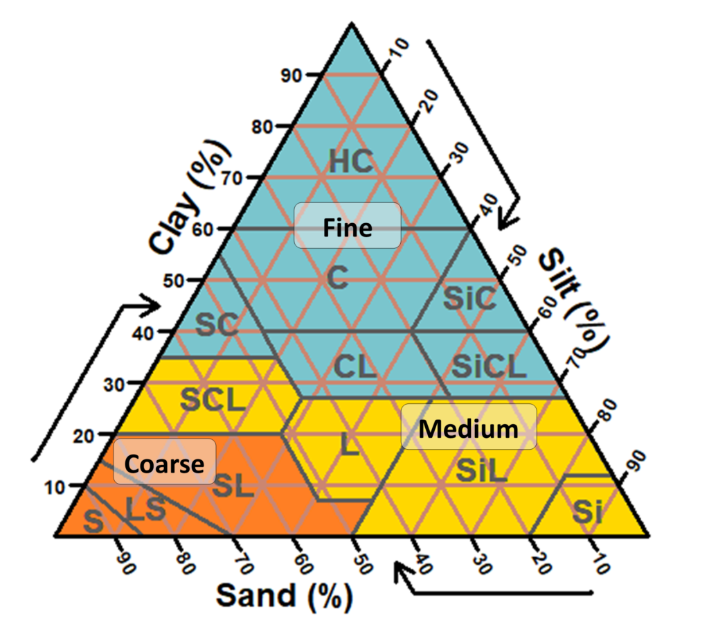
Select the texture that best describes the soil in the sample. Hand texturing is strongly recommended over relying on soil maps. The interpretation of SHAP depends on the texture category of the soil. Select a specific texture class if you can, otherwise classify the texture as sandy, loamy, or clayey.
To add another sample location within the same field (with the same management as described in the Soil Management Survey) click the plus icon ![]() at the bottom right of the page.
at the bottom right of the page.
Part 2 of the guidebook provides instructions for performing the in-field assessments and sampling.
Soil structure evaluations
If the Soil Structure Evaluation module was selected, use the Soil Surface Quality and VESS score sheets to assign scores to up to three subsamples within the sampling location. For each subsample, note the score and corresponding thickness of each layer in Survey123. If there are multiple layers, the weighted score will be automatically calculated. To add subsamples, click the plus icon ![]() .
.
Part 2 – What to do in the Field
This section of the guidebook will provide direction on symptoms to look for, as well as the specific steps for soil health assessment and sampling at the sample location.
Guidelines for in-field assessments and sampling
Timing
Soil health samples and observations should ideally be taken in the month of June, if possible. Soil moisture conditions are likely to be suitable for in-field assessments and soil biology has had to become active after winter, but conditions are typically not as hot and dry as in July or August, when biological activity can slow down again.
Avoid sampling after recent field activity (e.g., tillage or nutrient application) or if conditions are extremely dry or wet. Tilled soils need around 6 weeks after the last tillage pass to settle into a more representative physical condition.
Equipment
- SHAP submission form
- Soil sampling probe and small bucket
- Soil sample boxes and bags
- Smartphone / tablet for data entry*
- In-field Data Collection form*
- Shovel (for Soil Structure Evaluation module)**
- SSQ and VESS score sheets**
* if using SHAP Tool (Survey 123)
** if Soil Structure Evaluation module is selected
Sampling area for in-field evaluations
It is recommended to sample and evaluate from a specific point in the field – an area around 300 square feet – roughly a circle with a radius of 3 metres. If the field is split into homogenous zones, the soil sample can also be composited from this zone. Non-targeted sampling (i.e., traditional soil fertility sampling) is not recommended for SHAP as soil variability could limit the reliability of the interpretation.
Field observations
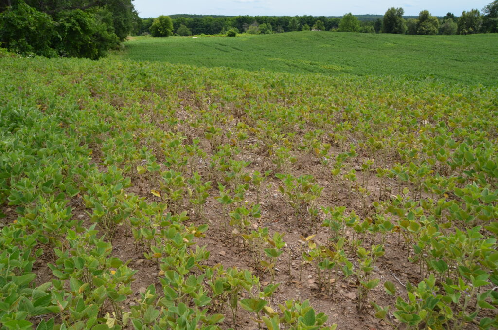
Although the suggested sampling protocol for SHAP is point-based, take the opportunity of visiting the field and walking to the sampling location to make general observations of the field. These could include differences in crop performance, localized deficiency, or disease symptoms, as well as soil erosion, soil colour, drainage, and compaction issues, and should be recorded as notes. For guidance on recognizing different types of soil erosion, see “Recognizing erosion symptoms in the field”.
Sample collection and submission
Collect 15-20 core samples to a 6-inch depth from within a 300 square foot sampling area(s). Remove surface debris and extract cores as you would for a normal soil fertility sample. Place cores into a clean pail. Gently break and mix the cores and transfer into standard soil sample containers.
Use soil from the composited sample to determine the texture. Consult the hand texturing guide if necessary. The sample must at least be classified as “sandy” (coarse), “loamy” (medium), or “clayey” (fine) for a soil health score to be calculated.
If the Soil Structure Evaluation module is selected, follow the instructions under Soil Structure Evaluation.
Packaging and shipping
Sample handling is important to get accurate best results from soil health tests. Keep samples out of direct sunlight, store them in a cooler, and ship them as soon as possible to a participating lab. Where samples cannot be submitted immediately, they should be refrigerated, but not frozen, for no longer than one week.
Once ready to ship, double bag the sample, place in an appropriate shipping container, and add packing material (e.g., crumpled paper or bubble wrap) if necessary to reduce sample movement. Add ice packs (inside their own plastic bags) if shipping during the hottest days of summer.
Make sure to include the SHAP submission form AND the lab submission form.
Participating Soil Testing Labs
As of April 2023, soil samples can be submitted to the following soil testing laboratories for analysis of the SHAP package:
Soil Structure Evaluation
Follow the instructions below to complete the Soil Structure Evaluation module. These assessments are best performed when the soil is moist (not too dry, but not wet), and at least six weeks following the last tillage event to allow the soil to settle to a more representative condition. This allows the soil structure and aggregation to be visible and representative.
Soil Surface Quality
To evaluate soil surface quality, refer to the SSQ score sheet. Select a score based on the description and photo that aligns closest to your observation. Repeat the assessment in three spots per sample location for the most representative result.
Soil Structure Quality
The Visual Evaluation of Soil Structure, or VESS, is a method to assess soil structural quality by comparing observations of soil aggregates and roots with a description chart to create a score. The method breaks down into three basic steps – soil removal, assessment, and scoring. The process should take no more than 20 minutes to perform per location. Refer to the VESS score sheet for detailed instructions and scoring guides.
Follow the instructions for soil removal and assessment on the first page of the scoring sheet. Match what you see to the descriptions and photos on the second page of the scoring sheet. Scores do not need to be whole numbers – intermediate scores of 1.5, 2.5, etc. can be assigned.
Repeat the assessment in three spots per sample location for the most representative result.
Hand Texturing
Soil health scores are calculated differently for fine-, medium-, and coarse-textured soils, so it is crucial for the soil to be classified into one of these soil texture groups at minimum. To determine the soil texture class, follow the flowchart and instructions below (reprinted with permission from “Characterizing Sites, Soils & Substrates in Ontario – Volume 1 Field Description Manual”. R.J. Heck, D.J. Kroestch, H.T. Lee, D.A Leadbeater, E.A. Wilson & B.C. Winstone).
Note: very fine sandy loam is included with Loam in the medium-textured group.

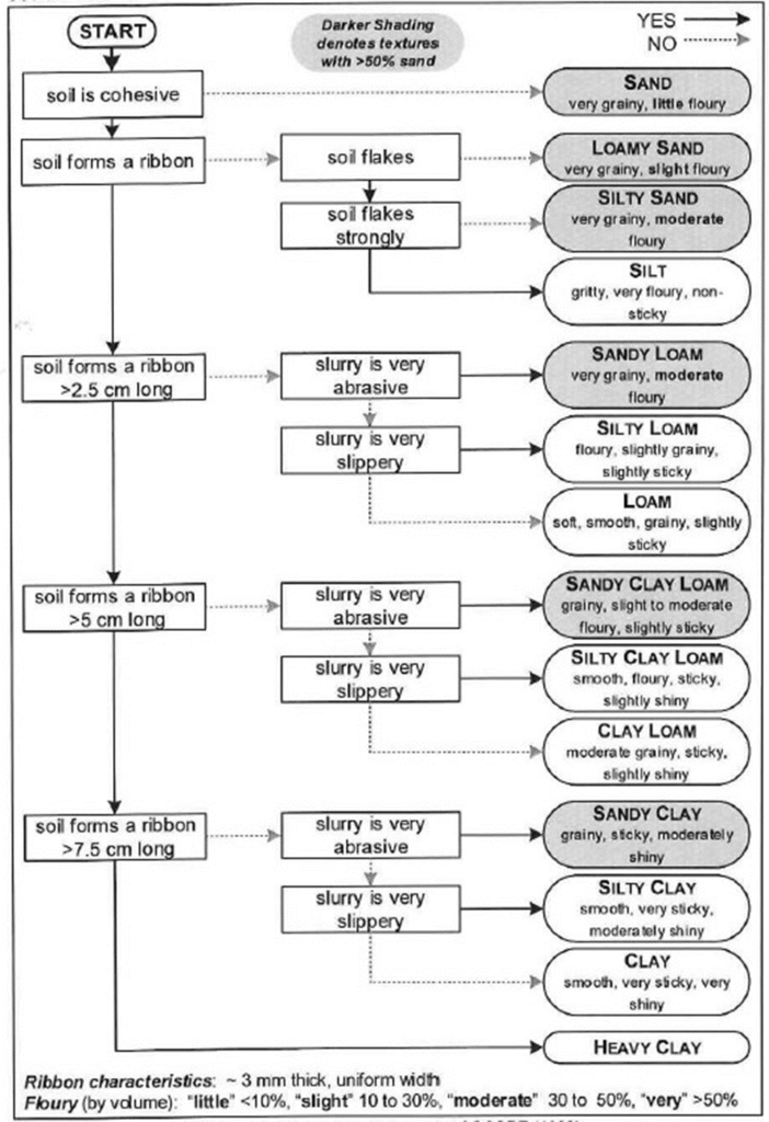
4.2.3 Field Assessment of Texture
4.2.3.1 Dry Feel Test
*For Soils with >50% Sand* Soil is rubbed in the palm of a hand, to dry it, then to separate and estimate the size of the individual sand particles. The sand particles are allowed to fall from the hand and the amount of finer material (silt and clay) remaining is noted (OCSRE 1993).
4.2.3.2 Preparation of Moist Soil for Hand-Texturing
Place about 1 golf ball volume of soil in the palm of a hand. Slowly wet and knead, removing any particles >2 mm. Soil is ready when it is plastic (see Section 5.4.2.3), but leaves negligible moisture when dabbed on skin.
4.2.3.3 Preliminary Moist Cast Test
Compress moist soil (see Section 4.2.3.2) by clenching it in a hand. If the soil forms a cast (holds together), test the strength of the cast by passing it from hand-to-hand, as well as by compressing it between thumb and forefinger.
| Cast Strength | Cast Characteristic | Textural Class |
|---|---|---|
| No cast | is not cohesive | S |
| Very Weak | does not withstand handling (lightly squeezing between thumb and forefinger, or transferring back and forth between hands) | LS, SiS |
| Weak | withstands careful handling (moderate squeezing between thumb and forefinger, or transferring back and forth between hands) | SiS, SL, Si, SiL |
| Moderate | can be readily handled | SCL, L |
| Strong | can be aggressively handled | SC, CL, SiCL |
| Very Strong | very resilient to handling | SiC, C |
4.2.3.4 Ribbon/Flake Test
Moist soil (see Section 4.2.3.2), is rolled into a cylindrical shape (~1 cm in diameter) that fits within a closed hand. Press the cylinder out between thumb and forefinger forming a ribbon of uniform width and thickness (~3 mm). Determine maximum length that is self-supporting against gravity. Silty soil will flake off the thumb, when rubbed against the forefinger.
4.2.3.5 Slurry Test
A pinch of moist soil (see Section 4.2.3.2), is placed into the palm of a hand. Water is added to slake (using finger) the soil into a thick slurry-a very abrasive slurry is indicative of sand; very slippery is indicative of silt.
4.2.3.6 Stickiness Test
Stickiness refers to the degree to which soil adheres to other materials. Soil is crushed in the palm of one’s hand; water is then slowly added to allow puddling. A pinch of puddled soil is pressed between the thumb and forefinger, and the degree of adhesion is observed as they are separated. Extra water or soil is added to the puddle to achieve maximum stickiness (point of evaluation).
| Stickiness | Description |
| Non-Sticky | practically no soil material adheres to the thumb and forefinger |
| Slightly Sticky | soil material adheres to both the thumb and forefinger, but comes off one or the other rather cleanly soil is not appreciably stretched when the digits are separated |
| Sticky | soil material adheres strongly to both the thumb and forefinger -tends to stretch somewhat -soil pulls apart, rather than pulling free from either digit |
| Very Sticky | soil material adheres strongly to both the thumb and forefinger -soil is notably stretched when fingers are separated |
4.2.3.7 Grittiness (Taste) Test
*Caution with Possible Contaminants* A small amount of soil is worked between the front teeth. Sand particles are recognized by a grainy “crunch”. Silt particles feel gritty, but do not “crunch”; individual silt grains cannot be felt. Clay is smooth with no sensible grittiness.
4.2.3.8 Shine Test
Using the moist soil (see Section 4.2.3.2), rub once or twice against a hard, smooth object (knife blade, auger handle, shovel) – any resulting shininess will increase with clay content.
Part 3 – Results Interpretation, Reporting and Planning
This part of the guidebook supports the final steps in the SHAP process. It explains the process for completing the SHAP report template, how the soil health scores are calculated, and how to complete the Soil Health Management Plan. A table of management options is provided with examples of actions that can be recommended in the plan. Finally, detailed sections for each soil health indicator explain how they are measured, how they are influence by management and other factors, and how to interpret them.
SHAP Report
Once both the Soil Management survey and the In-field Data Collection form have been completed and submitted, the submitter will receive an emailed SHAP report template containing the information gathered throughout the tool. A copy of the report template can be found here.
The submitter must complete the report by:
- Calculating scores with the SHAP Score Calculator and entering results in the summary table
- Providing an overview summary of the production practices, field observations, and soil health results.
- Completing the soil health management plan table with enough detail and justification to inform future management decisions.
Soil Health Scores
The approach to scoring individual indicators in SHAP is based on the Cornell Framework (Comprehensive Assessment of Soil Health, 3rd ed) developed by the foundational work of the Cornell Soil Health Lab. Normalized scores (converted to a 0-100 scale) allow for easy interpretation of measured values. Scores for analytical indicators are calculated by scoring functions that assign a score between 0 and 100 to the indicator values and are based on Ontario data. Scores for other indicators are based on established thresholds of soil quality or degradation risk. More detail on how these are calculated is provided in their respective subsections below.
Low scores suggest potentially limiting factors to soil health and productivity. High or very high scores indicate soils are functioning at the upper range of their potential in agricultural systems.
For easier visual interpretation, indicator scores are also assigned a color rating based on the Cornell Framework, as follows:
| Score range | Colour | Rating |
| 0-20 | red | very low |
| 20-40 | orange | low |
| 40-60 | yellow | medium |
| 60-80 | light green | high |
| 80-100 | dark green | very high |
Each soil health indicator is scored separately – there is no overall soil health score. Separate scores for individual soil health indicators give better direction for making management changes. The current state of soil health science does not support an overall score that averages the scores of each individual indicator as this would not account for relationships between indicators or for differences in relative importance between them.
Analytical Indicators
The scoring functions for analytical indicators in SHAP are created following the method developed for the Cornell Framework. Briefly, scoring functions are derived from soil health indicator values measured by laboratory analysis of Ontario soils by calculating the distribution of measured values in the scoring dataset for each indicator. As the scoring dataset expands, scoring functions will be periodically updated.
The Cornell Framework assumes results are normally distributed. For soil organic matter, respiration, and active carbon, the distributions of Ontario results were normal enough to apply this approach directly. Aggregate stability and PMN were not normally distributed, so data transformations were applied to enable scoring functions to be derived.
The results of most soil health indicators are strongly influenced by soil texture, and it would not be appropriate to directly compare the results for a loamy sand and a clay loam. To address this, the dataset for each indicator in the Ontario soil health dataset was analyzed. If the results from coarse-, medium-, and fine-textured soils (i.e., sandy, loamy, clayey) were different enough, they were grouped separately for determining the distribution curves.
These scoring functions allow for individual results to be compared to the range and distribution of results from similar soils in Ontario in addition to setting a baseline for a particular field. The resulting scores are like percentile scores – a score of 80 means that the result was higher than 80% of samples in the dataset it was compared to.
Soil health scores for a measured result can be calculated with a cumulative normal distribution function using the mean and standard deviation provided for each indicator. (Note: aggregate stability and PMN results must first be transformed.) The scoring function for each indicator is provided below for informational purposes. The SHAP Score Calculator performs these calculations.
Soil organic matter
Based on a dataset of 1841 samples, SOM is scored using separate functions for coarse, medium, and fine textured soils. The scoring curve, mean and standard deviation (in parentheses) for each texture group are provided below.

| Texture group | Mean (SD) |
| Coarse | 3.01 (1.07) |
| Medium | 3.77 (1.06) |
| Fine | 4.16 (1.12) |
Aggregate stability
Based on a dataset of 869 samples, aggregate stability could not be separated into different scoring functions. The scoring curve, mean and standard deviation (in parentheses) are provided below. These are based on the transformation WSA5.

| Texture group | Mean (SD) |
| All | 4.47 x 10⁹ (1.93 x 10⁹ ) |
Active carbon
Based on a dataset of 1802 samples, active carbon is scored using two separate functions: one for coarse textured soils and another combining medium and fine textured soils. The scoring curve, mean and standard deviation (in parentheses) for each texture grouping are provided below.

| Texture group | Mean (SD) |
| Coarse | 480 (156) |
| Medium & Fine | 588 (149) |
Respiration
Based on a dataset of 1219 samples, respiration is scored using two separate functions: one for coarse textured soils and another combining medium and fine textured soils. The scoring curve, mean and standard deviation (in parentheses) for each texture grouping are provided below.

| Texture group | Mean (SD) |
| Coarse | 14.5 (5.67) |
| Medium & Fine | 20.7 (5.89) |
Potentially-mineralizable nitrogen
Based on a dataset of 1827 samples, PMN is scored using separate functions for coarse, medium, and fine textured soils. The scoring curve, mean and standard deviation (in parentheses) for each texture group are provided below. These are based on the transformation PMN0.5.

| Texture group | Mean (SD) |
| Coarse | 2.62 (1.39) |
| Medium | 3.24 (1.32) |
| Fine | 3.50 (1.27) |
In-field Evaluations
Soil structure quality
The soil structure and soil surface quality evaluations are based on a five-point scoring scale ranging from sq1 (best) through sq5 (worst). The overall indicator values for these evaluations are averaged from all replications performed. In the case of the soil structure assessment, each replication is a weighted average of the score of the different structural layers present (see the VESS score chart pg 1). The evaluation scores are then normalized to 0 (worst) through 100 (best).
Soil structure quality score = 100 – (sq – 1) * 20
Management Evaluations
Tillage disturbance index
The Tillage Disturbance index uses the Soil Tillage Intensity Rating (STIR) system from the Revised Universal Soil Loss Equation (RUSLE2) to produce a quantitative rating of tillage disturbance. The STIR system was developed to quantify the impact of different tillage tools and systems on soil erodibility. It is calculated using the following equation:
STIR = 0.5(S) * 3.25T * D * A
Where S = speed, T = tillage intensity (based on the type of disturbance), D = depth, and A = the proportion of field area worked. The A factor is only relevant for tillage implements that do not disturb the soil for the entire width of the implement, e.g., strip-tillage, subsoiling, etc.
The scoring function was developed by plotting the STIR values of tillage systems representative of the range in Ontario field crop production. At the low end (STIR = 0) were 4-year hay crops and full no-till rotations. The high end (STIR = ~200) was represented by a corn – soybean rotation with fall primary tillage using a heavy disk, followed by secondary tillage using a light disk and two cultivator passes, with mechanical weed control by four in-season passes of an interrow cultivator working 70% of the field area. Four intermediate tillage systems of increasing intensity were also created for a total of 6 benchmarks to set the endpoints of the score ranges (0, 20, 40, 60, 80, 100). These broadly represent the tillage system descriptions from categorical scoring systems (e.g., Farmland Health Checkup) which could be named: “conventional”, “heavy reduced tillage”, “light reduced tillage”, “minimum tillage”, and “no-till/strip-till”.
The functional relationship between the STIR values and assigned scores was best captured by a linear equation with a breakpoint at STIR = 30.
Tillage Disturbance Index score =
for TDI <= 30, TDI score = 100 – 1.3333TDI
for TDI > 30, TDI score = 70.103 – 0.3605TDI
Living roots index
The Living Roots Index (LRI) calculates the proportion of days with roots in the ground. For each year, the number of days with living roots is defined as the difference in days between the planting of a crop or cover crop (whichever is earlier) and the harvest of a crop or termination of a cover crop (whichever is later). The LRI for each of the past 4 cropping years is averaged to create the LRI for the cropping system. The LRI score is then normalized to 100.
LRI score = (LRI/365) * 100
Risk Assessments
Water erosion risk
The Water Erosion Potential Map estimates water erosion risk based on soil type, topography, tillage system and crop rotation. It performs calculations from the Revised Universal Soil Loss Equation (RUSLE2) using data from the most recent soil maps for soil and landscape factors and calculates a ‘conservation’ (C) factor using tillage and cropping information provided.
This assessment produces a map of the erosion risk level, measured in tonnes per hectare, for each 10 x 10 m section of the field. These sections are defined by the resolution of the raster grid of soil and topographical variables from the Ontario Soil Survey Complex (i.e., digital soil maps).
The score for this indicator is based on the proportion of the field that is at elevated risk (defined as “moderate” (5 T/ha/year) or higher) of water erosion during the year when the crop that leaves the least surface residue is grown. The score decreases as this proportion increases.
Water erosion risk score = 100 – (% area moderate + % area high + % area very high)
Compaction risk
Terranimo assigns a risk rating to the scenario described by the input parameters based on whether the soil strength can tolerate the stress applied by the equipment. As the stress increases up to and beyond soil strength, the soil will deform, and compaction occurs.
Because there is no upper bound to this ratio it is not possible to assign a continuous numerical score. For that reason, compaction risk for the Spring/Planting and Fall/Harvest seasons is “scored” using discrete categories: Low, Considerable, and Excessive. The range of stress to strength ratios that fall into these categories is as follows:
| Risk Rating | Stress / Strength |
| Low | < 0.5 |
| Considerable | 0.5-1.1 |
| Excessive | >1.1 |
The Soil Health Management Plan
The Soil Health Management Plan is the key to providing value from the results of SHAP to the operation. A good plan integrates knowledge of the operation’s current management, objectives, and limitations with the results of the assessments conducted through SHAP. It recommends specific management actions that can be taken to address any concerns identified over the course of the assessment and includes enough detail in the considerations to ensure successful implementation.
The Management Options table provides examples of management actions and how recommended practices can be adopted over time. It can be used as a guide, but the final management plan must reflect the realities of the operation it is intended for.
| Management actions | Concerns addressed | Considerations |
| Early wins – high priority issues and/or low-hanging fruit (to implement next season) | ||
| Short term recommendations – incremental improvements towards more permanent solutions (2-5 years) | ||
| Long-term vision (5+ years goals) | ||
| Management actions | Concerns addressed | Considerations |
| Early wins – high priority issues and/or low-hanging fruit (to implement next season) | #colspan# | #colspan# |
| Short term recommendations – incremental improvements towards more permanent solutions (2-5 years) | #colspan# | #colspan# |
| Long-term vision (5+ years goals) | #colspan# | #colspan# |
| Management actions | Concerns addressed | Considerations |
|---|---|---|
| Early wins – high priority issues and/or low-hanging fruit (to implement next season) | ||
| blank | ||
| Short term recommendations – incremental improvements towards more permanent solutions (2-5 years) | ||
| blank | ||
| Long-term vision (5+ years goals) | ||
| blank | ||
Management options
The table below outlines categories of core practices that contribute to improved soil health. It provides rationale for each practice, along with a list of potential short, medium and long-term actions that can be undertaken. Every farm is unique; use this table – along with the findings from your soil health assessment – as a guide. Adopt new practices that fit the farm operation and farmer’s resources and skill sets. When combined, the practices detailed below can be synergistic and improve soil health significantly.
| Recommended Practice | Rationale | Actions |
|---|---|---|
| Reduce tillage intensity and/or frequency | • Decreasing soil disturbance is critical for diverse and active biological activity. • Intensive tillage temporarily stimulates certain microbes to decompose organic matter quickly. This reduces soil aggregation, promotes crusting and soil compaction, in addition to decreasing beneficial microbial activity. • Reducing tillage intensity can improve soil health and, over time, maintain or even increase yields, while reducing production costs due to saved labour, equipment wear, and fuel. | Short term • Reduce tillage to ensure a minimum of 30% soil cover (residue or growing crops) all year long • Leave residue cover later into the season before tillage (e.g., delay tillage after wheat harvest where cover crops are not an option, use alternate weed control options to allow tillage delay) • Adjust harvest equipment to spread chaff uniformly over full width of header • Manage cover crop termination to reduce need for tillage Medium term • No-till wheat after soybean harvest • Modify planting equipment to be capable of planting into spring residue cover • Avoid tillage after soybean harvest Long term • Plan crop rotation, residue management and equipment modification and/or replacement to enable reduced tillage e.g., strip till/no till |
| Diversify crop rotation | • Crop rotations can be as simple as rotating between two crops and planting sequences in alternate years or they can be more complex and involve numerous crops over several years (or at the same time) for improved soil health. • A diverse crop rotation is important for managing pests and balancing nutrient demand and is an important component of soil health management. • Ideal crop rotations generally increase species diversity and reduce pest pressure by interrupting pest life cycles through the absence of a suitable host or habitat. • Crop rotation can improve soil resiliency (to drought, extreme rainfall, and disease) especially after crops that usually involve intensive tillage. • Generally, yield increases when crops in different families are grown in rotation versus in monoculture (referred to as the “rotation effect”). • A cropping sequence for soil health management should include the use of cover crops and/or season-long soil-building crops. • Rotating a diversity of root structures (e.g., taproots and fibrous rooted crops from a variety of plant families) will also improve the soil’s physical, chemical, and biological health and functioning. | Short term • Investigate logistical and economic considerations of an additional crop(s) o Annual/perennial crop o Labour/equipment/workload timing o Weed control o Root systems/residue volume o Take low productivity or unprofitable land out of production (to plant trees/pasture) • Include a cover crop from a different family where a single crop is grown continuously. • Ensure past herbicide carryover will not affect planned crop or cover crops Medium term • Plan rotations that include winter cover as often as possible • Integrate a cereal crop (e.g. wheat, oats, barley) in rotation if not already present Long term • Include forage crops into the rotation • Include forage crops between orchard trees for potential grazing during periods of the year (while considering food safety) • Maximize pasture economics with rotational grazing • Establish agreements to “swap” fields with neighbours where diversified crop rotations are not practical |
| Integrate cover crops | • Cover crops provide a canopy, organic matter inputs, increased species diversity, and living root activity for soil protection and improvement between the production of main cash crops. They can be inter-seeded between some main crops. • Cover crops are grown as single species, or as mixes of two or many more species. • When used specifically to improve soil fertility, cover crops are also referred to as green manures. • The greatest benefits are usually achieved from cover crops that are terminated without tillage as this prevents soil disturbance and allows roots to decompose in the field and create continuous pores. • Cover crops contribute to soil organic matter through both above- and below-ground biomass. Root biomass is more effective. • Cover crops with fibrous root systems improve soil aggregation and alleviate compaction in the surface layer. • Cover crops with deep tap roots can help break-up compacted layers, bring up nutrients from the subsoil to make them available for the following crop, and provide access to the subsoil for the following crop via root channels left behind. • Cover crops can capture and recycle nutrients that would otherwise be lost through leaching during off-season periods. • Leguminous cover crops can fix atmospheric nitrogen that becomes available to the following crop. • Cover crops protect the soil from water and wind erosion, suppress soil-borne pathogens, and support beneficial microbial activity. • Dead cover crop material left on the soil surface can become an effective mulch that reduces evaporation of soil moisture, increases infiltration of rainfall, minimizes temperature fluctuations and aids in the control of annual weeds. | Short term • Determine goal(s) for cover crops, e.g. o Erosion control, N scavenging, N-fixing, building organic matter, breaking pest cycles, diversity o Determine where a cover crop can fit in the current crop rotation system Medium term • Determine adjustments necessary to include a cover crop in the current cropping system (e.g., herbicide concerns, termination plans, equipment modifications) • Start simple by seeding one or two species that winterkill following winter wheat harvest • Add complexity by including species with: o Diversified root systems and aboveground growth patterns o Over-wintering abilities o Fall/winter harvest/grazing potential Long term • “Swap” fields with neighbouring livestock producers to support grazing of cover crops • Where suitable, find methods to maximize growth of cover crop through earlier seeding (e.g., late-season inter-seeding in corn) or later termination (e.g., planting green with soybeans into cereal rye) • Make cover crops a consistent part of the cropping system |
| Add organic amendments | • Organic matter is critical for maintaining thriving soil biological communities, improving soil structure and root growth, increasing water infiltration, and building the soil’s ability to store and release water and nutrients for crop use. • Organic materials can be added by amending the soil with composts, animal manures, and crop or cover crop residues imported to the field from elsewhere. • The addition of organic amendments is particularly important in vegetable production where minimal crop residue is returned to the soil, more intensive tillage is generally used, and available land is limited. • Various organic amendments can affect soil physical, chemical and biological properties quite differently, so decisions should be based on cost, availability, composition, etc., and soil health and crop management goals. • Organic amendments derived from organic wastes should not only be tested for nutrients and pH, but also for micronutrients C:N ratio, EC or total salts and trace elements (heavy metals). • Manuring soil can increase total soil organic matter, cation exchange capacity and water holding capacity over time, and fresh un-composted manure, especially when solid, is very effective at increasing soil aggregation. Careful attention should be paid to the timing and method of application to meet the needs of the crop or crop rotation. • Use proper manure management practices to avoid nutrient losses to the environment, compaction, or pathogen concerns. | Short term • Look for nearby sources of manure or organic amendments o Consider nutrient content, organic matter contribution, logistics of transport and application, regulatory requirements (e.g., NASM plan), and economics • Take an analysis to determine nutrient content and reduce fertilizer rates accordingly • Avoid compaction o Avoid driving on wet soils o Hire custom applicators with central tire inflation systems (CTIS) o Apply to growing crops or undisturbed crop residue where possible o Minimize traffic to controlled traffic areas (e.g., traffic lanes, tram lines) Medium term • Avoid compaction o Purchase central tires inflation systems o Apply to growing crops or undisturbed crop residue where possible • Plan rotations so that amendments can be applied to fields further from the storage during the growing season • Use off-farm sourced organic amendments where manure is not available Long term • Plan to purchase application equipment that allows more flexibility for in-crop applications • Where fertility levels are high, sell or trade manure for straw • Consider de-watering, covered storages and other methods to reduce manure water content and reduce number of trips to the field |
| Prevent and reduce compaction | • Compaction damages soil structure by reducing soil pores, which constrains critical soil processes and important soil functions. • Soil compaction slows water movement into and through the soil. This results in slower soil warming and drying in the spring and increased risk of ponding and crusting. • Compacted soils have less available water capacity. As pores are destroyed, it takes less water to saturate the soil, and water content at field capacity is reduced. • Air, specifically oxygen, is just as important for crop roots as water. Both occupy the pores between soil aggregates. With reduced pore space, oxygen is reduced to growth-limiting levels at a lower water content. This inhibits root growth and creates conditions for root pathogens to thrive while limiting the beneficial microbial populations. • Roots grow through the soil by following existing pores or creating new ones by pushing soil particles and aggregates aside. In a dense, compacted soil this requires much more energy which is then not used for crop growth. When compaction is severe it can be too dense for roots to grow through, limiting the uptake and crop use efficiency of water and nutrients. • Compacted soils increase horsepower requirements for tillage and compromise seeding depth control and emergence uniformity. • For all the reasons above, compaction causes significant yield loss unless rainfall quantity and timing is perfect. This effect can last for several years, and deep compaction is essentially permanent. • Preventing compaction is much easier than fixing it, and generally cheaper. Compaction can be loosened through tillage and subsoiling up to a certain depth, but the effect is temporary unless the factors that caused it are changed. • The majority of compaction damage is caused by the first pass. Concentrating traffic to the smallest possible field area is better than spreading it out. • As traffic is concentrated, traffic lanes become more compacted, improving traction and fuel efficiency and reducing draft power requirements. Soil between the lanes will become more friable, improving tillage, seeding equipment, and drainage system performance as well as crop productivity. | Short term • Identify the high compaction risk scenarios and factors in the system and prioritize them for changes • As much as possible, wait until soils are a little dryer before performing field operations • Reduce tire inflation pressures to the minimum manufacturer recommendations when in the field • Verify that ballast weights are properly distributed and not higher than necessary • Set and follow the same A-B lines for equipment that makes multiple passes • Evaluate soil structure to identify compacted layers, and identify compacted areas in the field from crop growth patterns • During harvest, keep trucks on roads or headlands and drive buggies and wagons to headlands before heading to transport bins • Ask custom operators to follow as many of the above actions as possible Medium term • Focus on modifying the heaviest and most-used equipment to reduce compaction risk • Install central tire inflation systems (CTIS) to switch between road and field pressure • Replace old tires with types that can tolerate lower inflation pressure • Plan logistics of heavy field operations to reduce loads (i.e., don’t fill to capacity) • Develop an equipment replacement plan to enable semi-controlled traffic – equipment widths in multiples can mostly follow the same tracks (e.g., 90 ft sprayer boom, 30 ft planter, 30 ft combine header) • Modify equipment and/or cropping system to drive over cover crops or crop residue as much as possible • Plan rotations to avoid planting vulnerable soils to crops with damaging harvest operations (e.g., sugar beets) • Find custom operators who will respect your goals for compaction prevention Long term • Establish permanent tramlines and A-B lines for every field to concentrate traffic impact • Invest in tools and infrastructure for equipment guidance to enable traffic control • Replace equipment to fit the semi-controlled traffic plan o Consider how improved traction on established traffic lanes might reduce horsepower requirements • Evaluate how soil structure improvements might facilitate other soil health management practices (e.g., no-till, keeping residue cover into spring) |
| Build soil resilience | • Building resilient soils will help to maintain crops and feed for livestock during weather extremes associated with a changing climate. How soils, crops, and livestock are managed will have a role in determining the future pace of climate change, with implications for farming and food security. • Soil organisms, plants, and animals are important as both sources (producers) and sinks (absorbers) of greenhouse gases (GHG). • Building carbon in the soil with better soil management practices will help decrease the magnitude of CO2 and N2O emissions. • Improving water infiltration and drainage helps to minimize crop stress, topsoil loss, and flooding during extreme rainfall events. • Increased water holding capacity, in combination with better infiltration, allows for more water storage to buffer against short term drought. | • Reduce soil disturbance • Maximize carbon storage potential by combining practices, e.g., manure applied with cover crops to increase plant biomass. o Return straw/stover back to soil where possible • Include windbreaks and trees where possible for protection from wind erosion and longer-term carbon storage • Reduce the number of equipment passes per season • Utilize 4R practices with nutrient application o Band starter fertilizer o Inject side-dress fertilizers o Utilize nitrogen inhibitors where appropriate • Utilize organic amendments to reduce commercial fertilizer (nitrogen) inputs. o Test amendments to better estimate available nutrients • Where surface runoff and soil erosion are regular occurrences: o Consider erosion control structures (e.g., grassed waterways), in combination with reduced tillage and increased winter cover o Consider buffer strips along water courses |
Soil Health Indicators Explained
Soil Fertility
Soil fertility in an integral part of soil health. Sufficient nutrient availability helps to ensure high levels of crop productivity, which in turn returns large amounts of residue to the soil. This supports maintenance of soil organic matter and soil biological activity.
Recent soil fertility values are requested as a part of SHAP to ensure that important, productivity-limiting concerns are not over-looked, but it is outside of the scope of SHAP to provide detailed fertility recommendations. Use soil fertility information to guide decision-making for nutrient and lime applications, as required. Scoring of P and K values in SHAP reflect low, medium, and high likelihood of response ratings from official Ontario guidelines. Recommendations for lime application can be found in Publication 811, Agronomy Guide for Field Crops within the Soil Fertility and Nutrient Use chapter. Crop-specific fertilizer guidelines can be found within individual crop chapters of Publication 811 or the Crop Nutrient and Field Management tools of AgriSuite.
The following section provides information about the indicators used to measure soil health through SHAP. Understanding what an indicator measures, how that measurement is made, and how it relates to soil functions and processes is important to interpreting the results of soil health tests.
Analytical Indicators
Soil Organic Matter
Soil organic matter (SOM) is composed of materials associated with living organisms. It has an important influence on many processes in the soil. Soils with higher OM content have better structure, supply more nutrients to crops, and support greater soil biological populations, all of which make them more resilient to weather extremes. Changes in SOM content are slow to materialize, often taking several years to respond to management.
The percent SOM is measured by mass loss on ignition (LOI), which involves heating the soil sample in an oven at 500°C and measuring the change in mass. At this temperature, organic matter will burn off, leaving behind only the mineral soil and some ash.
Influencing Factors
SOM levels are influenced by inherent factors such as climate, landscape, and soil composition. Topography tends to influence variability in SOM levels across a field due to water availability, which affects plant biomass inputs to SOM, as well as redistribution by erosion of SOM-rich surface soil to lower slope positions. Soils with higher clay content tend to have higher SOM content. Clay surfaces provide better adhesion sites for organic matter to associate with minerals, and clay particles play a central role in the aggregation processes that protect organic matter from decomposition by microbes.
Relationship to Soil Function
SOM greatly impacts the physical, biological, and chemical properties of the soil and the processes they influence or result from. SOM is the primary food and energy source for soil organisms. Where it is protected from microbes, SOM acts as a long-term carbon sink. When it is exposed, it can act as a slow-release pool of nutrients, depending on its composition. It also contributes to the ion exchange capacity, which influences nutrient retention and availability. SOM is involved at every level in the aggregation process, which results in many of the soil’s physical properties. It also contributes to increased soil porosity, which is crucial to root growth and resource uptake, as well as to the soil’s ability to infiltrate and percolate water and exchange gases with the atmosphere. These benefits result in increase plant available water.
Interpretation
More SOM is better, and higher levels improve the soil functions mentioned above both directly and indirectly.
Management
The primary way that management influences SOM is through the relative rates of inputs (from photosynthesis) and outputs (decomposition and erosion). Very simply, when the balance is positive (more organic matter is input than output from the soil), SOM is likely to increase.
Biomass (from crops, cover crops, and organic amendments) is the primary input of organic matter. Consistent biomass additions are needed to feed microbial populations that convert biomass into SOM. But not all biomass is created equal, and the quality of the biomass influences how much of it stays in the soil. Recent research indicates that “high quality” (i.e., low carbon-to-nitrogen) biomass will result in a larger proportion of biomass carbon entering the slow-cycling SOM pool and increasing SOM levels over time.
Microbial populations will feed on any organic matter they can access, which makes physical protection of SOM inside of aggregates an important part of reducing losses. Tillage can destroy existing aggregates and disturb the aggregation process, exposing protected SOM to microbial decomposition. Conversion to no-till is one of the most widely recommended practice for increasing SOM. However, in the cold-temperate, humid to subhumid climate of Ontario, no-till alone does not consistently result in higher SOM levels in the full soil profile compared to conventional tillage. SOM benefits from no-till are more likely the longer the system is in place, as well as in fields with high erosion risk.
Active Carbon
Active carbon represents a fraction of soil organic carbon (about 1-4%) that is not the most microbially available (labile), but rather moderately stable and slightly processed. While it is strongly correlated to total soil organic carbon (SOC), it is most likely composed primarily of microbial metabolites including lipids and proteins that can be associated with soil minerals and thus protected from further decomposition. As it responds to management changes more quickly than SOC, active carbon can be interpreted as a leading indicator of future changes in SOC. Higher levels are associated with practices that tend to stabilize SOC and increase aggregate stability. This indicator is sometimes called “active carbon”, but with current understanding of what it measures that is misleading. Scientists usually refer to it as permanganate-oxidizable carbon, or POXC.
This indicator measures how much of the SOM in the soil sample can be oxidized by a 0.2M concentration of potassium permanganate (KMnO4) when shaken for 2 minutes. The quantity of organic matter that reacts with KMnO4 changes the colour of the solution, which is measured with a spectrometer and compared to standards of known concentrations.
Influencing Factors
Active carbon levels are influenced by soil moisture and temperature, which affect the rate of mineralization of SOM. Soil drainage class can also influence active carbon, as very poor drainage results in anaerobic conditions that can lead to losses of organic carbon as methane (CH4).
Relationship to Soil Function
Active carbon is positively related to the benefits that come with healthy soil biology, particularly with respect to transformations of organic matter.
Interpretation
Like with total soil organic matter, more is better when it comes to active carbon. If repeated sampling shows a decrease in active carbon, it may signal declining SOM levels, and vice versa. There is some indication that comparing active carbon to mineralizable C (i.e., respiration) can provide insight into the direction of SOM trends, but more work is needed.
Management
Practices that are known to increase SOM will also increase active carbon. Consistent carbon additions from organic amendments and cover crops are likely to increase active carbon, as are reductions in tillage intensity.
Respiration
Soil respiration is a measure of potential carbon mineralization and an indicator of biological activity. Many soil microbes feed on SOM, releasing nutrients and other compounds that benefit plants and influence other soil processes. As they metabolize that SOM, they respire some of it as CO2. The amount of CO2 released is related to the quantity of available carbon in SOM, as well as to the population and activity levels of microbes that consume it.
Respiration measures the amount of CO2 released from an oven-dried and re-wetted soil sample at room temperature over four days. Re-wetting a dried sample re-activates microbes and often breaks aggregates, exposing previously protected SOM. This results in an initial flush of CO2 that then tends towards an equilibrium after a few days.
Influencing Factors
The activity of soil organisms varies throughout the season, and even daily, in line with soil conditions such as temperature and moisture. Respiration rates in the field are affected by temperature and moisture at the same time, especially whichever is the most limiting. Soil temperature affects the rate of microbial processes such that respiration roughly doubles for every 10°C increase, up to a maximum of 35-40°C, beyond which microbial activity and respiration decline. At the other end of the thermometer, microbial activity essentially stops below about 5°C. Respiration typically increases with soil moisture until water-filled pore space starts limiting oxygen availability. As soils dry, respiration declines due to lack of moisture required for biological activity. While it may be slightly variable between sites, the ideal moisture content is around field capacity.
Soil texture, pH, and the quality and quantity of organic matter also influence respiration by impacting moisture availability, soil organism activity and carbon sources available to microbial populations.
Relationship to Soil Function
Respiration is an integrative measure of the abundance and activity of biological life in soil. It reflects the status of primary producers (e.g. plants and algae) and most consumers (e.g. decomposing bacteria and fungi, and the organisms that eat them). Respiration can be related to all the functions these organisms provide, such as breaking down plant residues, converting nutrients in organic matter into forms that are plant-available through mineralization, storing carbon and nutrients in microbial biomass and building soil structure.
Interpretation
Generally, more is better when it comes to respiration, and higher CO2 levels can be related to larger and more active biological communities with access to plenty of food sources. Higher respiration rates indicate that residues will be broken down more quickly, and that the nutrients contained within them will be made available for crops. Very high respiration rates, however, may indicate excessive SOM mineralization in the short term, and declining SOM levels in the longer term. Excessive respiration usually occurs after tillage, as the destruction of soil aggregates exposes previously protected SOM. Generally, low organic matter levels, poor soil structure, and nutrient limitations result in low respiration values.
Management
Biological activity measured by soil respiration can be limited by the supply of SOM as a food source or by other constraints to growth. Practices that increase the supply of SOM and improve the quality of the soil as a habitat will enhance respiration.
Food sources for soil microbes include crop residue, cover crop biomass and exudates, and organic amendments. A consistent supply is important. This can be accomplished through crop rotation that includes a winter crop or a perennial forage, including cover crops whenever possible, and applying organic amendments.
The habitat quality of the soil is improved by the SOM-enhancing practices above, but also by reducing disturbance from tillage. Compaction avoidance practices and proper drainage will maintain the diversity of aggregate sizes and pore spaces where soil organisms live, and maintain a proper balance of air and water in those pore spaces.
Heavy metals, salts, and some plant protection chemicals (pesticides, fungicides, and herbicides) can have a negative impact on soil organisms.
Potentially Mineralizable Nitrogen
Potentially Mineralizable Nitrogen (PMN) measures how much of the nitrogen tied up in organic matter can be converted (mineralized) into plant-available ammonium under certain temperature and moisture conditions over time.
Potentially mineralizable nitrogen measures the change in ammonium (NH4) content after incubating the fully saturated soil sample at 30°C for 7 days. Saturation creates anaerobic conditions that limit the conversion of NH4 to NO3 so that the difference in NH4 after 7 days can be entirely attributed to ammonification, where N-containing organic compounds are broken down into NH4.
Influencing Factors
PMN is mainly influenced by soil type, landscape, and SOM. Soil texture influences PMN in much the same way as it does for respiration. As organic nitrogen is a part of SOM, aggregation processes that make it unavailable to microbes will limit its contribution to PMN. Potentially mineralizable nitrogen levels will also generally track with SOM content across a field. Higher levels of both are likely to be found in lower or depressional areas that accumulate SOM and total N. Accumulation and mineralization of N also depend on the carbon-to-nitrogen ratio of materials added to the soil. Lastly, PMN is also dependent on the abundance and activity of microbial species that can convert organic nitrogen into ammonium.
Relationship to Soil Function
PMN relates to the soil’s capacity to supply crops with nitrogen, as well as to microbial growth and activity. While soils often contain large reserves of total N, most of it is in the form of organic molecules and not directly available to plants. PMN indicates how much of that total N is readily available for conversion and the capacity of soil microbes to perform that conversion under favourable moisture and temperature conditions.
Interpretation
PMN levels can be used as an estimate of potential soil N supply during the growing season. When it comes to soil N supply, more is generally better. However, in the absence of growing vegetation or in wet conditions, large amounts of mineralized N could be vulnerable to loss to groundwater through leaching or to the atmosphere via volatilization or denitrification. Because the incubation uses specific conditions, it may not exactly reflect what will happen in the field and should be combined with other measures of soil N such as soil nitrate for in-season management decisions.
Soils with depleted organic matter will likely have a low PMN value.
Management
Beyond the weather-dependent factors of temperature and moisture, the rate of soil N supply depends on the size of the organic N pool. Stocks of organic N in the soil can be increased by adding organic amendments rich in organic N, such as manure. Plant biomass with low carbon-to-nitrogen ratios (e.g., legume cover crops) will also increase soil organic N, both directly and via microbial biomass built up as they decompose.
The other way to improve PMN is through building microbial populations. In addition to providing them with high-quality, consistent food sources, providing suitable habitat in the form of neutral pH and good soil structure will support strong microbial populations.
Aggregate Stability
Aggregate stability refers to the resistance of soil aggregates to disintegration following disturbance. It indicates how well aggregates can resist tillage, raindrop impacts, and water erosion.
The aggregate stability test involves placing a sample on top of a stack of progressively finer sieves and moving it up and down in water. As aggregates break down (slake) they fall through to smaller sieves. Results are shown as the percent of stable macroaggregates (>0.25mm). A correction is made for sand and gravel (particles >2 mm). More, larger stable aggregates indicate better, more resilient soil structure.
Influencing Factors
Aggregate stability is influenced by clay content, as clay particles play a central role in the aggregation process. Clay particles expand and contract and they moisten and then dry, creating cracks in the soil that can create, break apart, or rearrange aggregates.
Organic matter and biological activity drive aggregation at multiple scales. Aggregates often form around pieces of organic matter. Earthworms create aggregates by bringing organic matter and soil particles together in casts, as well as by secreting mucus that coats and further binds aggregates together. Roots and thread-like networks of fungal mycelium connect and bind small aggregates into larger aggregates and may also produce some binding agents. Some by-products and dead cells of other organisms also act as binding agents or form bonds between organic compounds and mineral particles that connect aggregates.
Specific cations are important in the formation of microaggregates and in determining their stability. Calcium, magnesium, iron, and aluminum form bridges between negatively charged organic matter and clay particles. Sodium (and, to a lesser extent, potassium) is negatively related to aggregate stability, and high levels of sodium ions between soil particles promotes dispersion of aggregates.
Relationship to Soil Function
Stable aggregates are the result of many beneficial soil processes, and the foundation of good soil structure. Aggregate stability is positively related to organic matter content, biological activity, and erosion resistance.
Stable aggregates are the building blocks of good soil structure. Well-aggregated soil has high porosity, which is key to the soil’s ability to infiltrate, percolate, and hold water, as well as exchange gases with the atmosphere. Smaller pores within macroaggregates hold plant-available water at field capacity. Large pores between large aggregates facilitate water and root movement through the soil, as both water and roots tend to follow the path of least resistance. Large pores connected to the surface accelerate infiltration, which decreases runoff and erosion risks. Well aggregated soil is more resilient to weather extremes as it holds more plant-available water between permanent wilting point and field capacity and drains more easily.
Unstable aggregates disintegrate during rainstorms, filling surface pores and drying into a crust. This reduces infiltration, leading to runoff, water erosion, and reduced water storage and availability in the soil. It also restricts oxygen flow into the soil and obstructs seedling emergence, which increases plant stress and susceptibility to disease. Low aggregate stability leads to poor soil structure, reduced porosity, and increased compaction, making it more difficult to manage.
Interpretation
Greater amounts of stable aggregates indicate better soil health. Soil health also tends to increase as the proportion of large aggregates increases. Large macroaggregates (>0.25mm) are more sensitive to management as they are composed of microaggregates (0.25-0.002 mm) weakly bound together. Changes in aggregate stability may serve as early indicators of recovery or degradation of soils, as the process of aggregation involves proper functioning of biological, chemical, and physical processes.
Management
Improving aggregate stability requires a combination of reducing disturbance and increasing SOM and biological activity.
Stable aggregates require time to form, and tillage can disrupt that process, as well as destroying existing aggregates and structures such as fungal hyphae that tie them together. Any reduction in the frequency and intensity of tillage operations will benefit aggregate stability. Aggregates can also be destroyed by pounding rain, by abrasion from wind-blown soil particles, and from compaction. Keeping a consistent cover of residue and plants will protect aggregates from these impacts and supply the food source and microclimate required by the organisms that help build them.
Any practice that increases SOM will improve aggregate stability. This includes additions of organic amendments, though aggregates form especially well in the presence of fibrous roots. Cover crops with extensive fibrous root systems produce many root hairs that stimulate macroaggregate formation directly through physical action, but also indirectly by feeding soil microbes with root exudates and by encouraging mycorrhizal fungi to expand their hyphal networks. The most well-aggregated soils tend to be those under permanent perennial grass cover.
In-field Assessments
Soil Surface Quality
The soil surface is the interface between the soil and the atmosphere. Its quality – roughness, porosity, stability – determines the rates of exchange of water and gases. Visual assessment of soil surface quality can give an indication of soil health and soil function. A soil surface that has plenty of residue cover, presence of earthworm casts, and a rough, granulated structure will function much better than one that is sealed off.
Influencing Factors
Weather and soil texture are the strongest factors influencing soil surface quality, after management. If the soil surface is bare, raindrop impact can destroy surface aggregates. The dispersed microaggregates and soil particles settle into surface pores, sealing them and forming a crust. Clay content influences aggregate stability, and crusts on clay soils can crack more easily as they dry, mitigating their impact on gas and water exchange to some extent. Silty soils have very fragile aggregates and can easily crust. Sandy soils do not easily form aggregates, but sealing is rarely an issue because the size of sand particles creates enough space between them.
Interpretation
With good surface quality, water can infiltrate into the soil, but also evaporate from it. Oxygen – needed for respiration by roots and microbes – can diffuse into the soil, and byproducts such as CO2 and ethylene are able to leave it.
Soil with poor surface quality is more susceptible to crusting. This reduces infiltration, leading to runoff, water erosion, and reduced water storage and availability in the soil. Crusting also restricts oxygen flow into the soil and hampers seedling emergence, which increases plant stress and lowers crop stands.
Management
The surest way to improve soil surface quality is to maintain consistent surface cover of residue. Living cover (e.g., from an overwintering crop or cover crop) substantially improves surface quality by moderating the soil microclimate. Soil surfaces under a plant canopy are buffered from extreme fluctuations in temperature and moisture, which creates a more hospitable environment for crop roots and soil life. Crop residues on the surface provide a habitat and food source for soil organisms that improve aggregation at the surface. Soil organic matter improves aggregate stability, and practices that increase SOM will improve soil surface quality and function.
Tillage has a negative impact on surface quality because it reduces soil cover and can weaken soil aggregates. Any reduction in tillage will also increase earthworm populations, specifically those of deep burrowing, anecic earthworms that deposit rich, stable casts at the surface, and whose burrows are the best channels for water, air, and crop roots in the soil.
Soil Structure
Soil structure is an excellent indicator of soil health because it is the result of physical, biological, and chemical processes in the soil, and it has a strong and obvious relationship to crop productivity. Structure describes both the aggregates in the soil and the spaces between them.
Influencing Factors
Clay content influences aggregation, so structure tends to be more clearly defined as clay content increases. Cycles of wetting and drying (or freeze-thaw) contribute to defining structure as aggregates shrink and swell, creating cracks between them.
Interpretation
The Visual Evaluation of Soil Structure (VESS) rates soil structure quality on a 5-point scale. The table below provides a description of each score – from best to worst – along with a photo example.
| VESS Score | Example |
| Sq1 – Undisturbed grass fencerows will often exhibit this quality of soil structure, though it is also possible for well-managed cropland. | 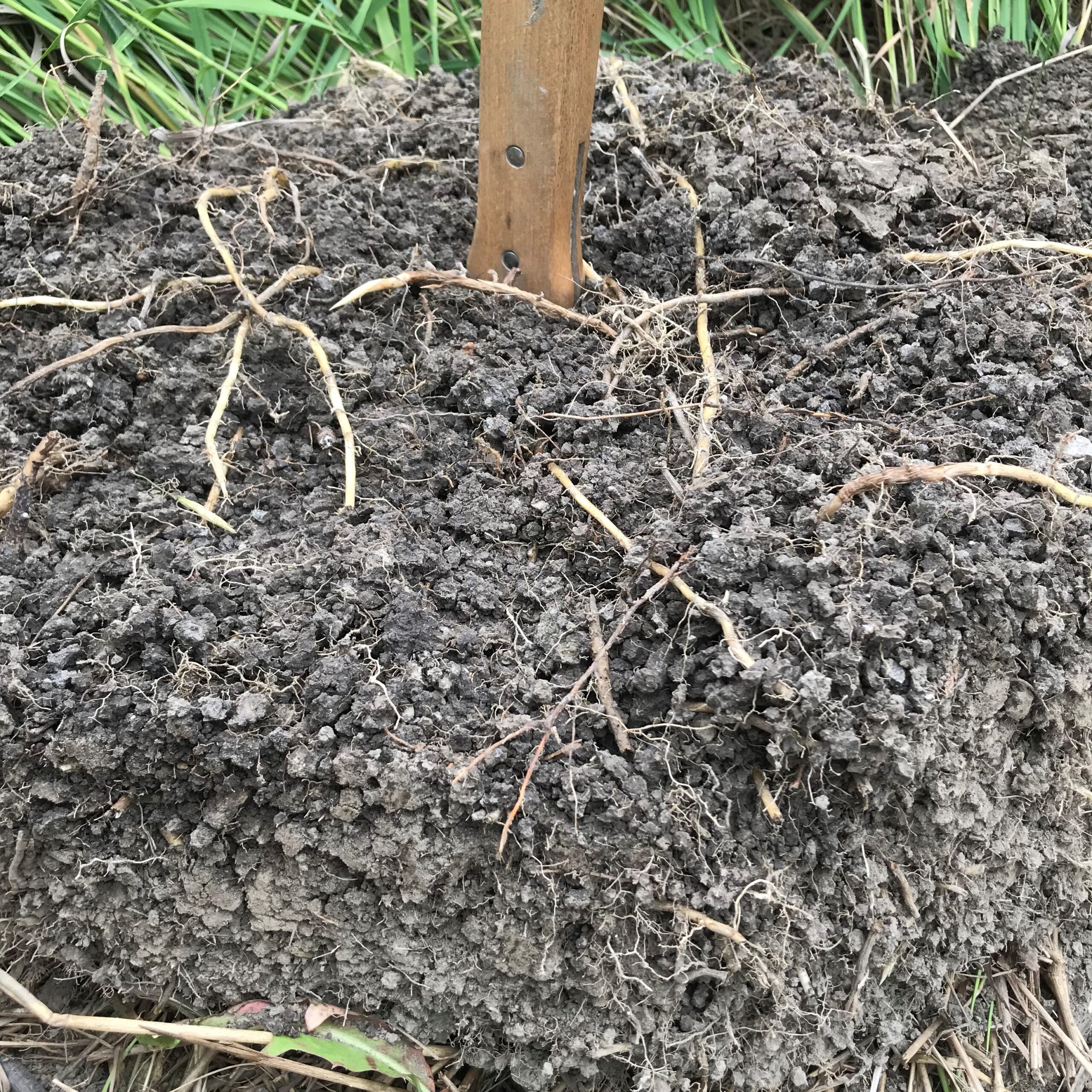 |
| Sq2 – More often found in good, well-managed cropland soil. Maintenance and compaction avoidance are the only management needed. | 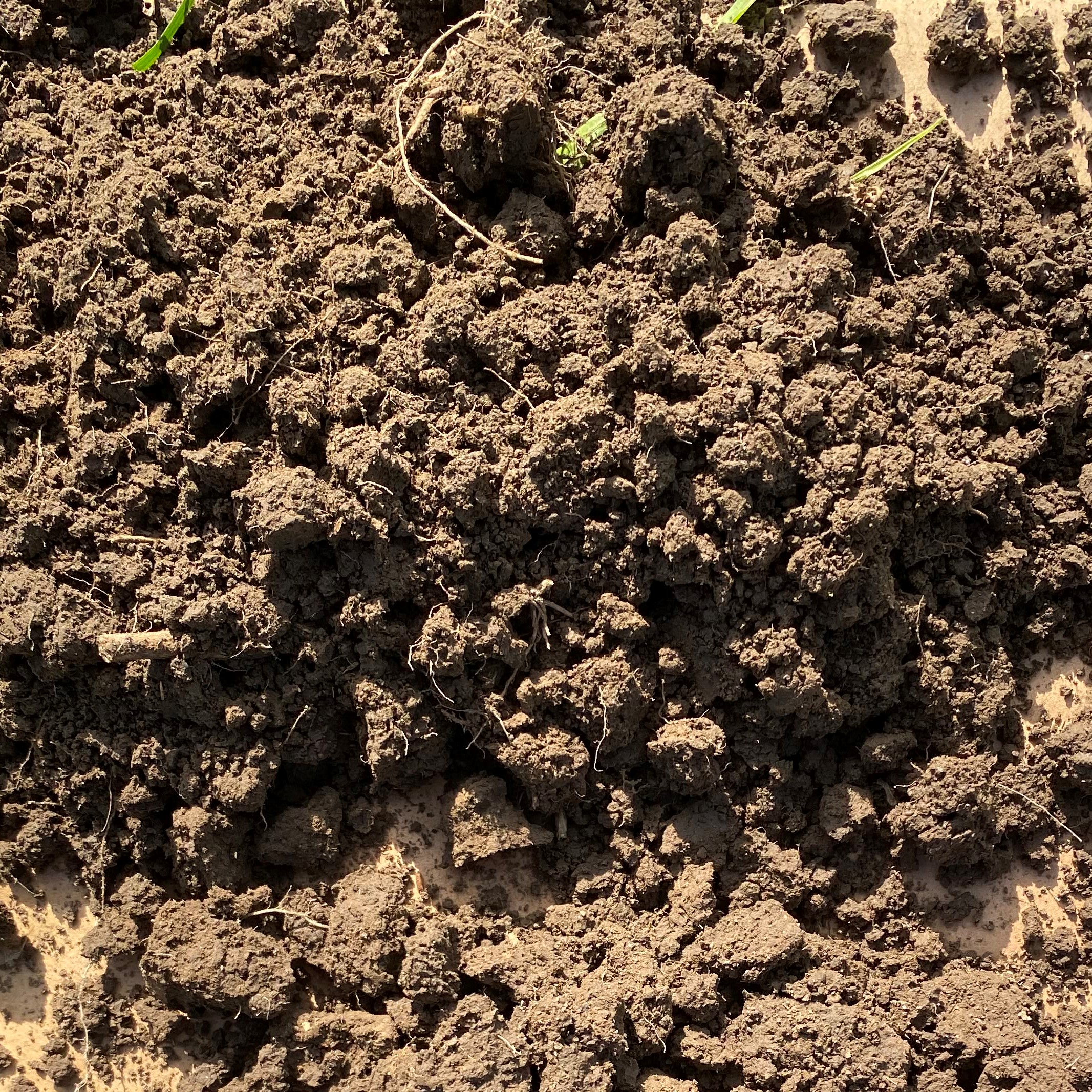 |
| Sq3 – Structure-based limitations on soil functioning may start becoming apparent. Much of the spadeful is cloddy (larger, compact chunks) with limited porosity. These soils should be improved by management. | 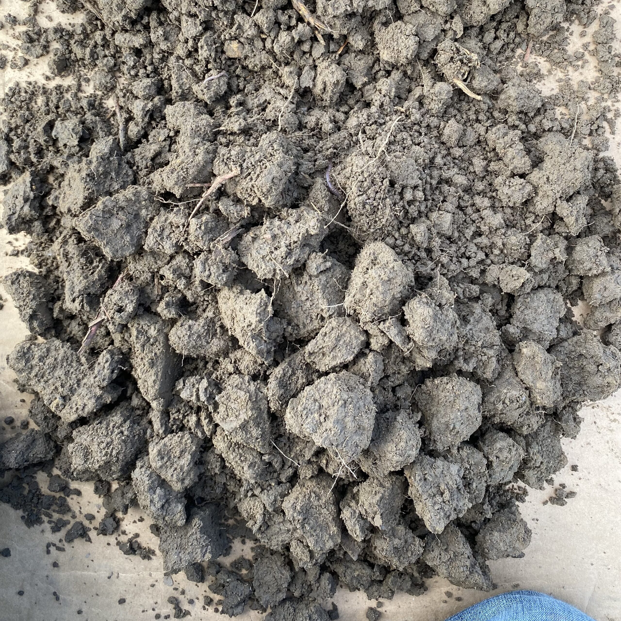 |
| Sq4 – Compacted soils will usually result in a score of Sq4. These soils should be improved by management, and mechanical loosening should be considered. | 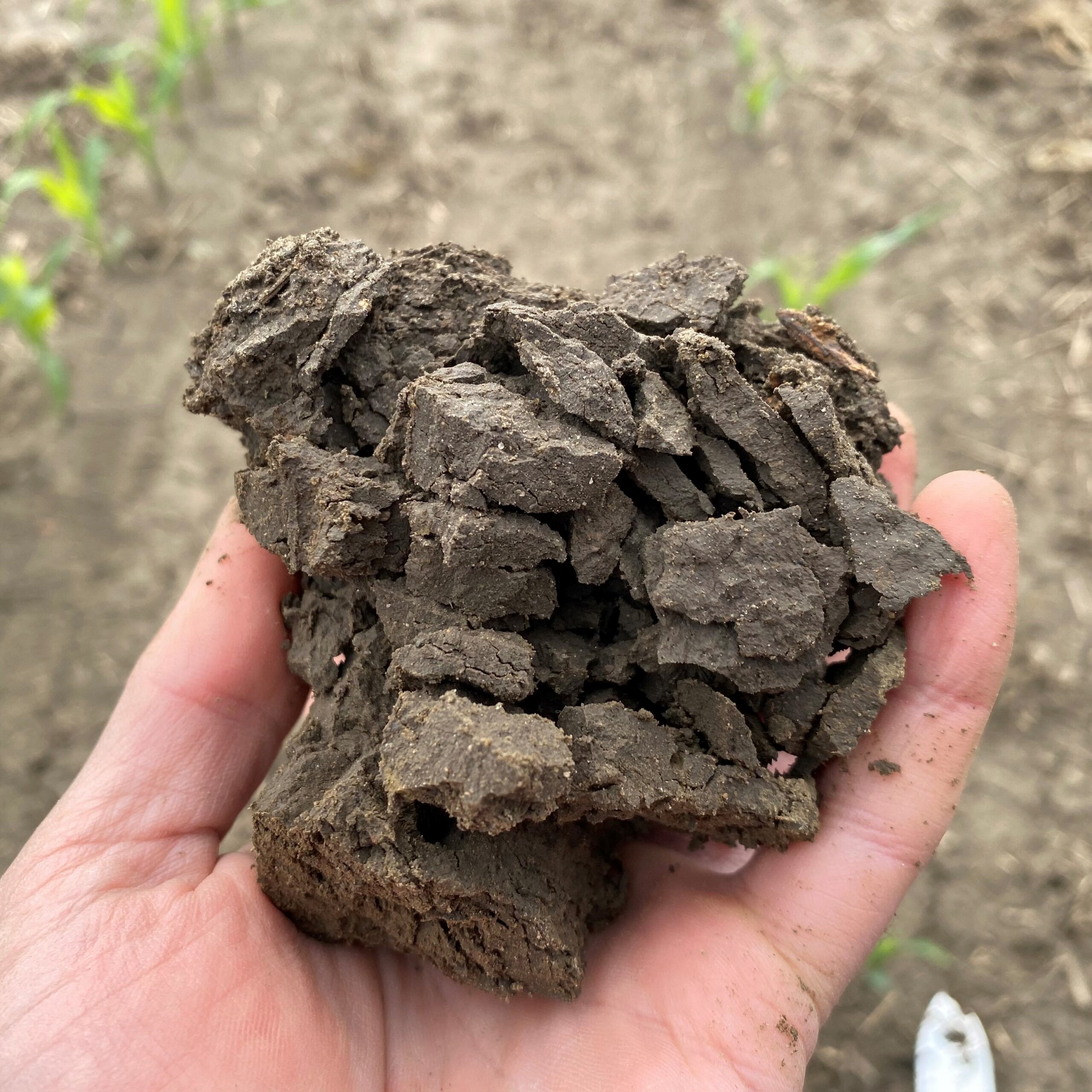 |
| Sq5 – When a score of Sq5 is reached, mechanical loosening is often required to break up large clods and re-establish a more favourable soil structure that can then be stabilized through management. | 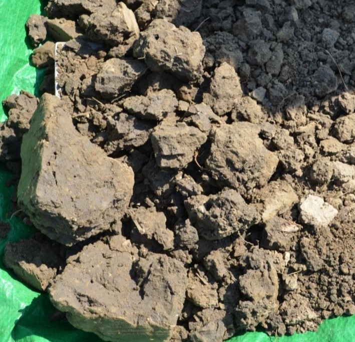 |
Many soils have at least two distinct layers of different soil structure quality. The top-most layer typically exhibits better soil structure, as secondary tillage and seedbed preparation, high root density, and freeze-thaw cycles all act to remediate surface compaction. The depth of this layer usually corresponds to the depth of secondary tillage, though the layer may also be found in perennial grass stands in the absence of tillage.
In some soils the opposite pattern may be found – surface soil may be more compacted than the layer below. In these cases, the soil stress (pressure exerted on the soil) was enough to compact the surface but did not extend to the layer below. This pattern can be found in grazing situations, or on farms with small, light equipment. In rarer cases, different layers of soil structure can be partially caused by differences in soil texture with depth.
Soils with higher clay content typically have blockier soil structure and more angular aggregates in the subsoil. To evaluate whether a blockier second layer is due to compaction or natural pedological processes, it helps to dig deeper. If a second 8” spade depth from the bottom of the first pit reveals better structure, the culprit is compaction. If not, it could be natural.
VESS is currently not well adapted for sandy or gravelly soils.
Management
Root action improves aggregation by providing organic matter for aggregates to form around. Like freeze-thaw cycles, roots also induce wet-dry cycles that cause aggregates to swell and shrink, creating or continuing cracks in clods and larger aggregates.
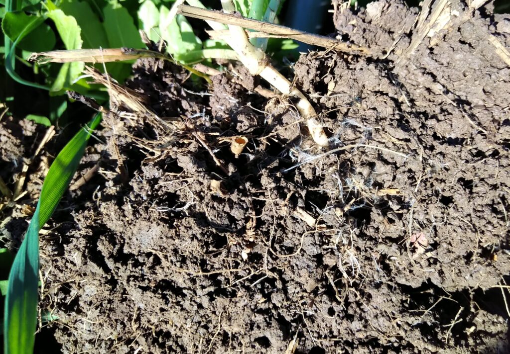
In contrast, tillage breaks up aggregates. While incorporation of organic matter (e.g., plant residues) could provide sources for aggregates to form around, tillage disrupts the cycle of aggregation whereby organic carbon becomes protected in smaller aggregates.
Reducing tillage and increasing the quantity and time of roots in the soil will improve aggregation, as will the consistent addition of organic amendments. Solid sources are best for improving structure.
Soil porosity – especially connected, continuous macroporosity – is a crucial element of soil structure that is less easily observable. Surface residue is the only food source for the types of worms that create continuous macropores. Maintaining surface residue and reducing tillage provides them with food and keeps their burrows intact.
Risk Assessments
Water Erosion
The water erosion risk assessment module uses the Water Erosion Potential Map tool in AgMaps. This tool calculates sheet and rill erosion from water for each 10 m2 pixel across the field. It uses the Revised Universal Soil Loss Equation 2 (RUSLE2) to estimate annual soil loss.
Influencing Factors
Average annual soil loss is influenced by rainfall, soil erodibility (from soil texture), slope gradient and length, soil cover, tillage, and any existing erosion control practices.
Interpretation and management
The “Inherent Water Erosion Potential” output estimates annual soil loss if the field were kept bare year-round – it excludes the soil cover and erosion control factors and shows the inherent erodibility based on climate, soil, and landscape factors. The “conservation” (C) factor is calculated from the combination of crop and tillage type. Adding this factor to the equation results in the “Mean Annual Water Erosion Estimate”.
There are clearly more factors that determine erosion in a field than the current crop and tillage method. The C factor should ideally be calculated for the entire rotation, and organic matter levels and compaction status will influence how much water infiltrates or runs off. The tool currently does not include these capabilities, nor does it calculate gully erosion, though these will be included in future updates.
See the table below for guidance on understanding erosion rates and management options to address them.
| Water erosion risk category | Mean Annual Water Erosion Estimate | Interpretation |
| Very low | <2 t/ha (<1 t/ac) | These categories are considered “sustainable soil loss”. The loss of soil due to water erosion is small. However, even small amounts of annual erosion can add up over time. If the field is losing > 1 t/ac/year, consider practices that will protect soil over winter during vulnerable portions of the crop rotation, e.g. seeding a winter cereal following soybeans or corn silage, reduced tillage or residue management . |
| Low | >2-5 t/ha (1-2.2 t/ac) | |
| Moderate | >5-10 t/ha (2.2-4.5 t/ac) | Even if it is not obvious, areas of the field at and above this soil erosion level are losing so much soil that they will not be able to sustain current production levels economically into the future. These areas should be considered high priority for targeted erosion BMP implementation, e.g. reduced tillage, winter crops and cover crops. |
| High | >10-18 t/ha (4.5-8 t/ac) | High rates of erosion will likely be obvious to see in spring. Although rills may be tilled and filled in, this only masks the problem – soil is being lost at a high rate. Implement no-till practices, till and plant crops across slope where possible and seed cover crops. Consult an expert as to whether structural erosion control measures would help in addition to agronomic practices. |
| Very high | >18 t/ha (>8 t/ac) | The topography, soil type and tillage and cropping practices are causing excessive soil loss from water that will severely limit yields and increase production costs. In addition to the cultural erosion control BMPs listed above, structural erosion control solutions like berms and grassed waterways are needed. Consult with an erosion control contractor to design and construct these structures. |
Soil Compaction
Soil compaction is an increase in the density of the soil. Compaction happens when forces applied to the soil (soil stress) exceed the soil’s capacity to withstand them (soil strength), leading to deformation. Compacted soils are denser, with less pore space for air and water exchange, and fewer large macropores for roots and water to follow. The consequences often manifest as slow drainage and ponding from limited water infiltration and percolation rates, drought susceptibility because of reduced available water capacity, and crop stress from nutrient deficiencies and disease due to impeded root growth and low-oxygen conditions.
The compaction risk assessment module asks the user to calculate subsoil compaction risk for the most vulnerable parts of the field at the most vulnerable times of year – i.e., highest clay content soils in spring and fall, when soils are most likely to be very moist and field operations are time sensitive.
Influencing Factors
Soil stress is the product of factors including load, tire inflation pressure, and contact area. Soil strength is difficult to measure, but is affected by clay content, moisture content, and soil structure.
Types of compaction
Surface compaction occurs in the top several centimetres of soil. It relates primarily to tire inflation pressure and contact area. Wheel slippage and sidewall compaction may also be present in this layer, but these are smearing actions rather than compaction.
Subsurface compaction is generally found at the depth of the deepest tillage pass. A zone of higher density and larger clods extends 10-30 cm below this. A “plow pan” caused by smearing may or may not be present, but an abrupt change of structure is usually evident.
Subsoil compaction most commonly affects the soil near the transition layer between A and B horizons, typically around 30 cm from the surface. While lower tire inflation pressure and greater contact area may spread the impact, axle load is by far the dominant factor at this depth
Interpretation and management
Terranimo uses equipment weight (input as wheel load) and tire inflation pressure to estimate soil stress at 35 cm depth. Clay content and water content are used to estimate soil strength. The compaction risk level is assessed based on the ratio of soil stress to soil strength.
| Compaction risk | Stress / Strength | Interpretation |
| Low | < 0.5 | Current equipment is unlikely to cause subsurface compaction damage in these conditions |
| Considerable | 0.5 – 1.1 | Current equipment is likely to cause subsurface compaction damage – equipment and/or timing needs some adjustment |
| High | > 1.1 | Current equipment is very likely to cause severe subsurface compaction damage – equipment and/or timing needs major adjustment |
If the ratio of stress to strength indicates elevated risk of subsoil compaction (>0.5), changes need to be made to either reduce stress or increase strength. The compaction avoidance options flowchart below outlines how SHAP helps to determine which combination of changes will result in low risk, in order of general acceptability to most operations.
Tire pressure is easiest to change, though investment in upgrades (e.g. wider, more flexible tires or CTIS) might be needed.
Soil moisture can be reduced only with patience, unless there are problems with the drainage system. But spring and fall field operations are time sensitive and can’t reasonably be delayed past a certain point. That point was defined as the water content at 90% available water: 12 cbar for sandy (coarse) soils, 23 cbar for loamy (medium) soils, and 23 cbar for clayey (fine) soils.
Reducing wheel load (the weight of equipment when loaded divided by the number of wheels) is the only option left if tire pressure and soil moisture can’t be reduced any further. This can be achieved by a combination of proper ballasting (minimum ballast required for efficient operation), filling equipment to below capacity, and adding more wheels or axles.
Concentrating traffic to the smallest possible area of the field will reduce the risk of compaction regardless of soil conditions and equipment setup. The majority of compaction damage is caused by the first pass. Keeping traffic on the same wheel tracks spares the rest of the field from compaction damage and limits the risk to established traffic lanes. Complete Controlled Traffic Farming (CTF) systems usually require modifying equipment to match axle widths, but “semi-CTF” systems can accomplish much of the same benefits without such drastic measures. The key is to use the same traffic lanes for all operations and match equipment working widths in multiples so they mostly follow the same tracks (e.g., 90 ft sprayer boom, 30 ft planter, 30 ft combine header)
Management Assessments
Tillage Disturbance Index
Tillage is the main way soil is disturbed in production systems. The primary way this disturbance affects soil health is by disrupting soil structure and reducing surface cover. Among other consequences, these effects increase the soil’s vulnerability to erosion. Reduced soil cover and weakened soil structure increase the speed of water runoff and the amount of soil that is susceptible to being carried with it.
The Tillage Disturbance Index module provides a quantitative measure of the intensity of tillage disturbance to the soil over the crop rotation. It uses the Soil Tillage Intensity Rating (STIR) system developed for the Revised Universal Soil Loss Equation (RUSLE2) to quantify the impact of different tillage tools and systems on soil erodibility. It is calculated for each cropping year and then averaged over the rotation.
Influencing Factors
STIR is calculated using the following equation:
STIR = 0.5(S) * 3.25T * D * A
Where S = speed, T = tillage intensity, D = depth, and A = the proportion of field area worked. Tillage intensity is a factor based on the primary action of the implement.
| Tillage types | T factor |
| Inversion, some mixing | 1 |
| Mixing, some inversion | 0.8 |
| Lifting and fracturing | 0.4 |
| Mixing only | 0.7 |
| Compression | 0.15 |
The STIR system currently does not properly account for powered implements (e.g., rototillers, power bedders, power spaders etc.). These will be added once this limitation is addressed. In the meantime, consider these implements to be highly disruptive and destructive in terms of soil structure.
Interpretation and management
In general, less disturbance is better for soil health. Beyond erodibility, tillage intensity negatively affects aggregate stability and the stabilization of carbon by physical protection within aggregates.
However, tillage can be an important for successful and profitable crop production in some circumstances. The goal should be to reduce tillage intensity and frequency to the minimum required for the production system. Use the cropping-year index results to identify opportunities in the cropping system to reduce tillage intensity. For example, consider whether certain crops could be grown with less tillage than currently used, or whether changes to the cropping sequence or rotation could reduce the tillage requirements for establishing subsequent crops.
Living Roots Index
The Living Roots index (LRI) module provides a measure of the average number of days per year with living roots in the soil.
Influencing Factors
Climate is the main factor determining these dates in most cases, and warmer climates with longer seasons have a clear advantage.
Because it is calculated from the past 4 cropping years (as opposed to a theoretical cropping sequence), the cropping system LRI can vary within a given rotation based on the starting point. For example, in a strict corn-soy-winter wheat rotation, starting with the wheat year leads to a higher LRI because two winter wheat years are included where only one is included if starting with the corn or soybean years.
In most cases the index will overestimate true living root days. Many crops are harvested significantly later than the physiological maturity of the plant, when roots stop growing and are arguably no longer alive.
Interpretation and management Roots are central to building soil health. Root exudates feed beneficial microbes in the rhizosphere that provide services to the plant and contribute to building soil carbon, and root biomass is more efficiently converted to soil organic matter than shoot biomass. Roots also contribute to improving soil structure, infiltration, and drainage. Fine roots and mycorrhizal filaments build stable macroaggregates, and channels created by roots are important conduits for water flow. All things equal, more days of root growth translates to more roots providing these benefits more consistently through
Forms and Resources
SHAP Submission Form
Use this form to list the soil samples sent to the lab for soil health analysis and to record the critical metadata for interpretation (soil texture) and for future resampling of benchmark or baseline sites (date, type, location). This is especially critical if not using the SHAP Tool for in-field data collection.
Note: Submit this form IN ADDITION to the lab’s usual submission form recording your contact and payment information. Contact the lab for this form.
SHAP Report
The SHAP report template can be downloaded from the link below. Users of the SHAP Tool should not need to download this file – upon submitting the In-field Data Collection form they will receive an emailed template with input fields automatically filled from information entered into and calculated by the SHAP Tool.
SHAP Scoring Calculator
Recognizing erosion symptoms in the field
Before heading to the field, review the Water Erosion Potential Map generated through AgMaps from the Water Erosion Risk module if it was selected. It will help you identify areas of concern and guide in-field observations.
Looking for erosion after tillage and planting in the spring can be difficult. Often delaying the visit until after a rainstorm will help to see patterns, particularly rills and sheet erosion.
Water Erosion
Water erosion happens when soil particles are moved downslope by rain impact or runoff. That soil will either be deposited in a lower landscape position or carried into surface water and leave the field entirely. Look for evidence of surface water movement within the field and from adjacent fields. Clues can include areas where crop residue and fine soil particles accumulate (low spots), or areas of concentrated water flow, which can form gullies. There are three major types of water erosion: sheet, rill, and gully erosion. Each looks and acts differently and should be addressed differently as well.
Sheet erosion occurs when water flows more or less evenly over the surface. While the quantity of soil particles lost can be substantial, it is usually difficult to notice visually.
Rills form when runoff begins to concentrate. They appear as shallow, typically parallel gouges on the slope.
Gullies form when runoff quantity and concentration is higher than with rills and are often seen where rills and/or slopes converge. A gully is “ephemeral” if it is small enough to be masked by tillage. When larger, a gully is considered permanent.
Refer to the table below for in-field visual symptoms and examples of each form.
| Water erosion type | In-field visual symptoms | Examples |
|---|---|---|
| Sheet | A buildup of soil and/or residue at the bottom of the slope or where slope decreases/flattens out No apparent rills or gullies May observe small stones held up by small columns of soil where soil has been eroded | 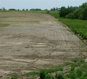 |
| Rill | Parallel, linear patterns on slopes Clear path where water has been flowing May see some exposed stones/rocks | 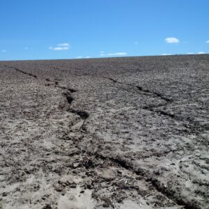 |
| Gully | Deep cuts in soils along slopes Clear path where water has been flowing A permanent gully is so large that equipment cannot travel over it | 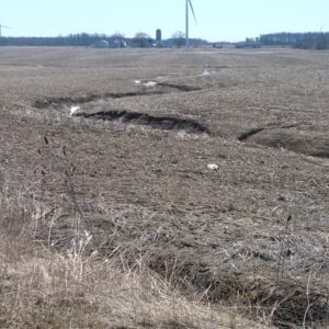 |
Wind erosion
Wind erosion is most easily observed during the winter and early spring in Ontario. It occurs most often on light-textured soils and on flat fields with minimal residue cover that are exposed to prevailing winds.
| Time of year | Symptoms | Examples |
|---|---|---|
| Winter | Dirty snow (“snirt”) Small drifts or accumulation of soil especially along ditches | 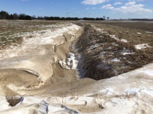 |
| Spring | Small drifts or accumulation of soil especially on the leeward side of any type of barrier, e.g. fence rows, buildings, trees, ditches or streams The soil surface appears smooth or rippled, like beach sand. May see small stones or chunks of residue left perched on a column of soil. |  |
| Crops may have been exposed, sandblasted or buried by soil | 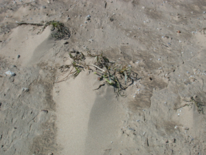 |
Tillage erosion
Tillage erosion occurs when tillage re-distributes soil from high slope positions to lower slope positions. It is aided by gravity, which moves soil particles down-slope, and takes place gradually over many years. Tillage erosion moves topsoil off the very tops of knolls, where it is then more susceptible to water erosion. This form of erosion is especially common on fields with complex topography.
It is helpful to check topsoil depth across slope positions. You may observe a very shallow layer of topsoil on knolls along with very deep topsoil in low slope positions. The image below shows the impact of tillage erosion on topsoil colour and depth, as well as soybean growth.
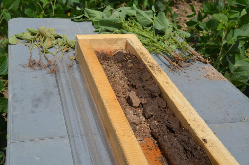
The following symptoms can be used to identify the occurrence of tillage erosion:
- Exposed subsoil or parent material
- Evidence of erosion on shoulder slopes of hills or whitish caps/sides of slopes
- More erosion evident than expected based upon soil types and slope
- Poor crop growth on the tops of knolls, particularly in dry seasons (image below)